

The Tails Run the Market
How left-tail risk and right-tail optionality shape investing
🔍 Executive summary
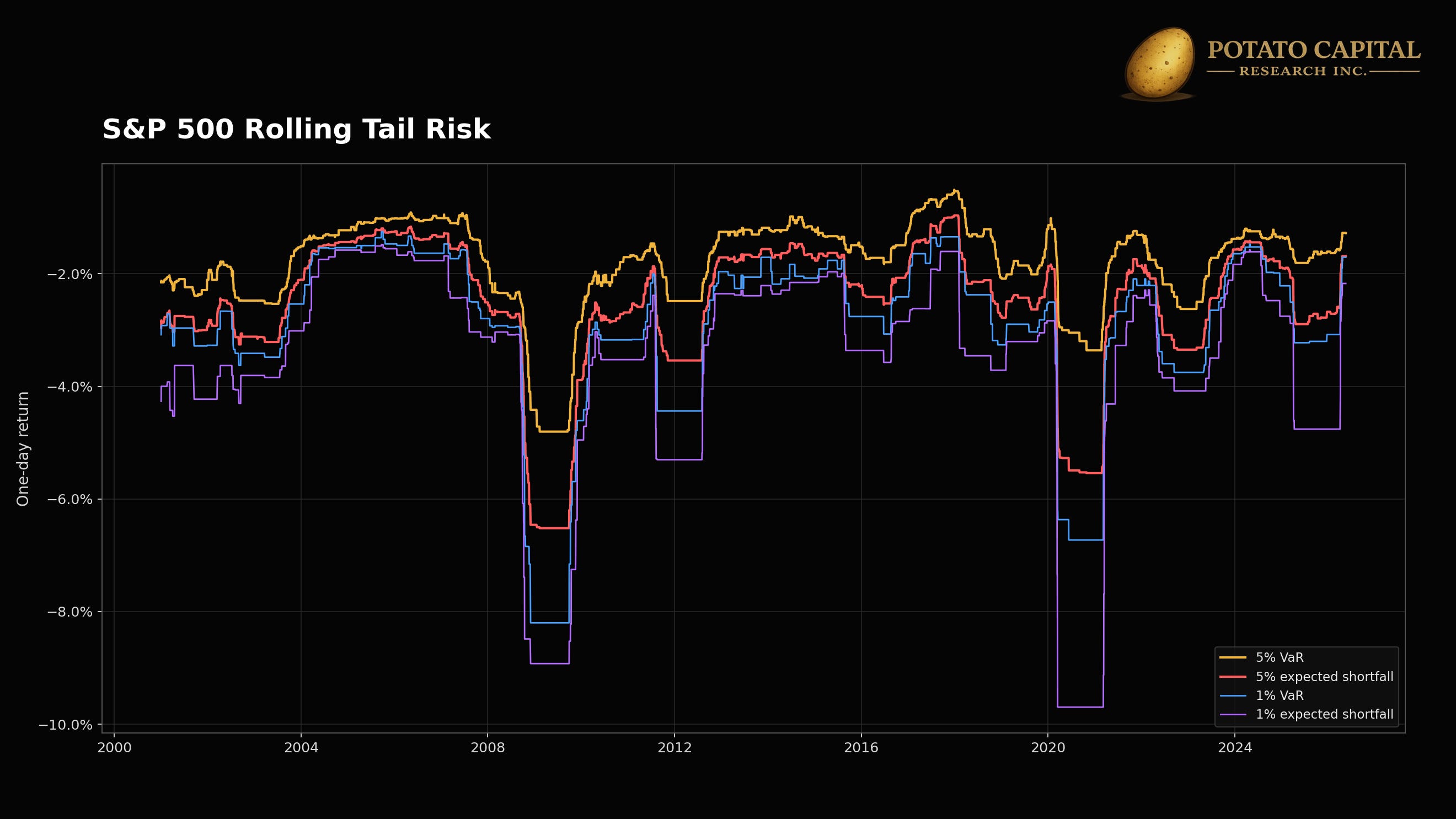
The long-run average hides the part investors actually have to live through. Since 2000, the S&P 500 daily price series annualized at 6.4%, but the path included fat-tailed daily losses, a -56.8% maximum drawdown, and repeated regime shifts. The 1% Value at Risk cutoff was -3.4%, while expected shortfall inside that worst 1% bucket was -4.9%, which is the cleaner measure of what capital actually had to survive.
The left tail becomes permanent when losses force action. Credit spreads raise refinancing costs, duration can fail when inflation and rates rise, and elevated margin debt adds forced-selling fuel if volatility, credit spreads, and equity drawdowns begin moving together. The current market is not showing broad systemic stress, but it has clear vulnerabilities: downside skew remains present, QQQ carries wider implied path risk than SPY, margin debt is elevated, and long-duration assets remain sensitive to higher long rates.
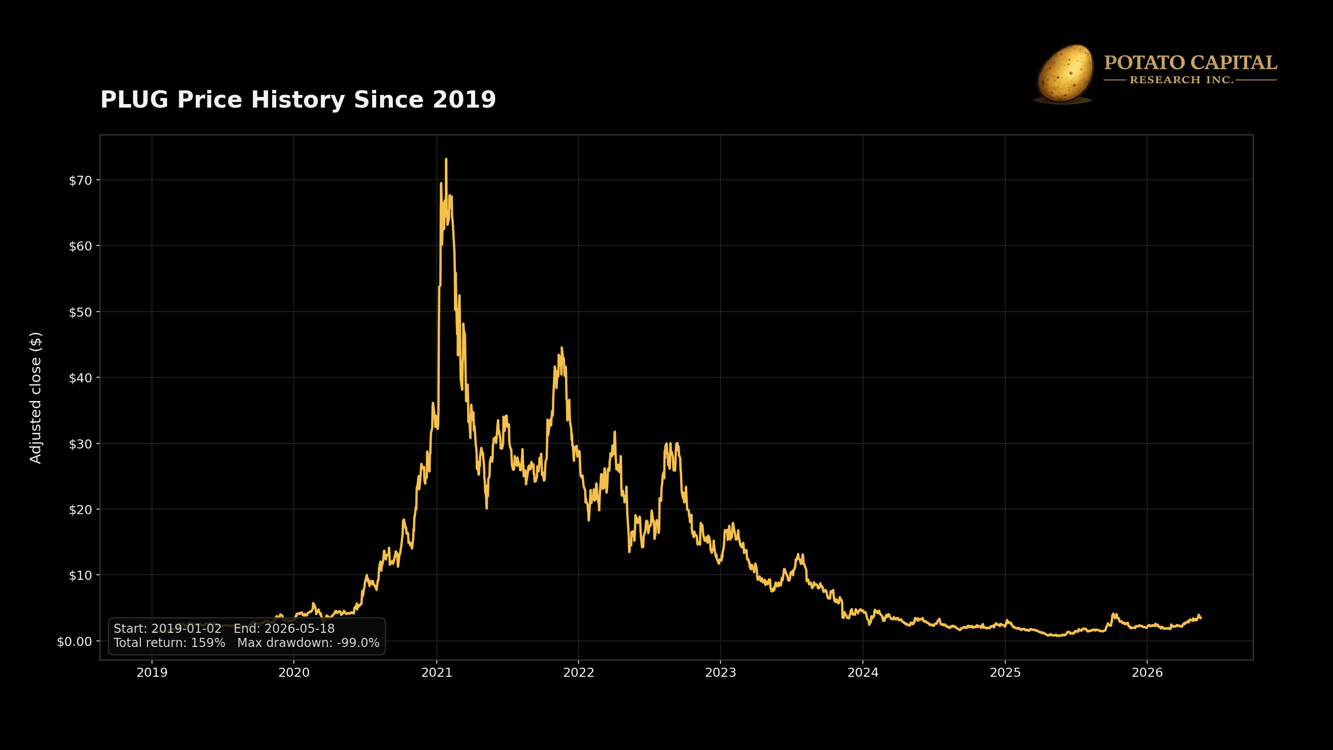
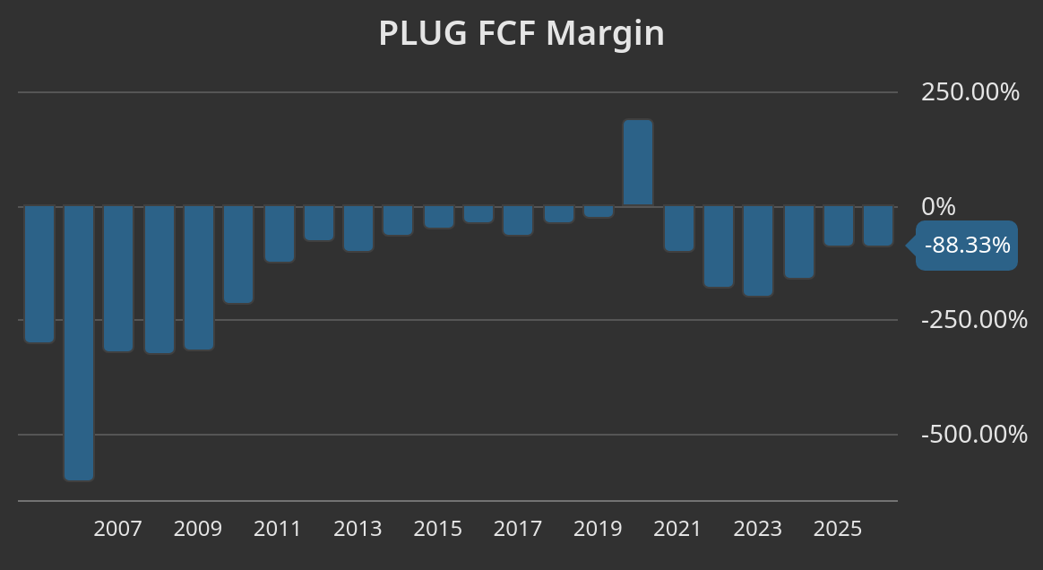
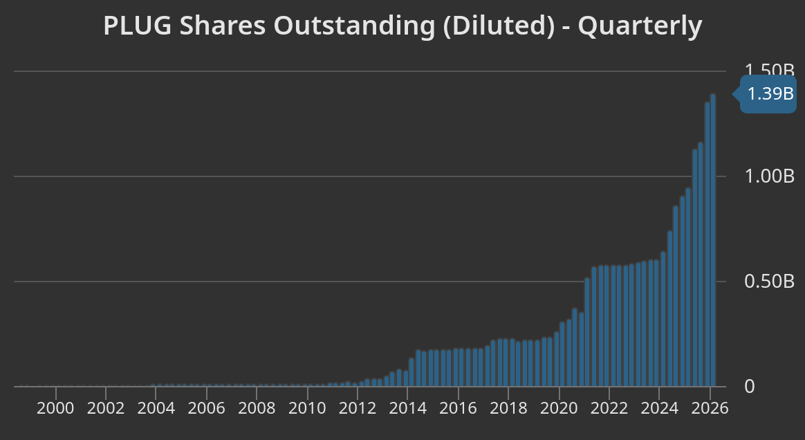
The right tail also needs discipline. NVDA and META show higher-quality optionality because growth converted into free cash flow and shareholder capture. PLUG and BYND show the failure case: revenue narrative without durable cash economics or dilution control. CVNA and FCX show that distressed recovery and commodity torque can produce large payoffs, but the drawdown path requires tighter sizing.
Valuation, hedging, and position sizing all need to be distributional. A multiple is only useful if it is tied to cash conversion, dilution risk, balance-sheet risk, and scenario probabilities. Hedges need to match the shock being hedged: duration for recessionary disinflation, real assets for inflation or supply stress, index protection for broad beta, and cash for liquidity. The real question is which tail the portfolio is being paid to hold, whether the price is reasonable, and whether the position size can survive the path required for the thesis to work.
📊 The Average is Not the Experience
Since 2000, the S&P 500 daily price series annualized at 6.4% with 19.3% volatility. That is the summary after the fact. The actual path included the dot-com unwind, the global financial crisis, the COVID shock, the 2022 inflation and rate reset, and several smaller volatility spikes that get compressed inside the long-run average.
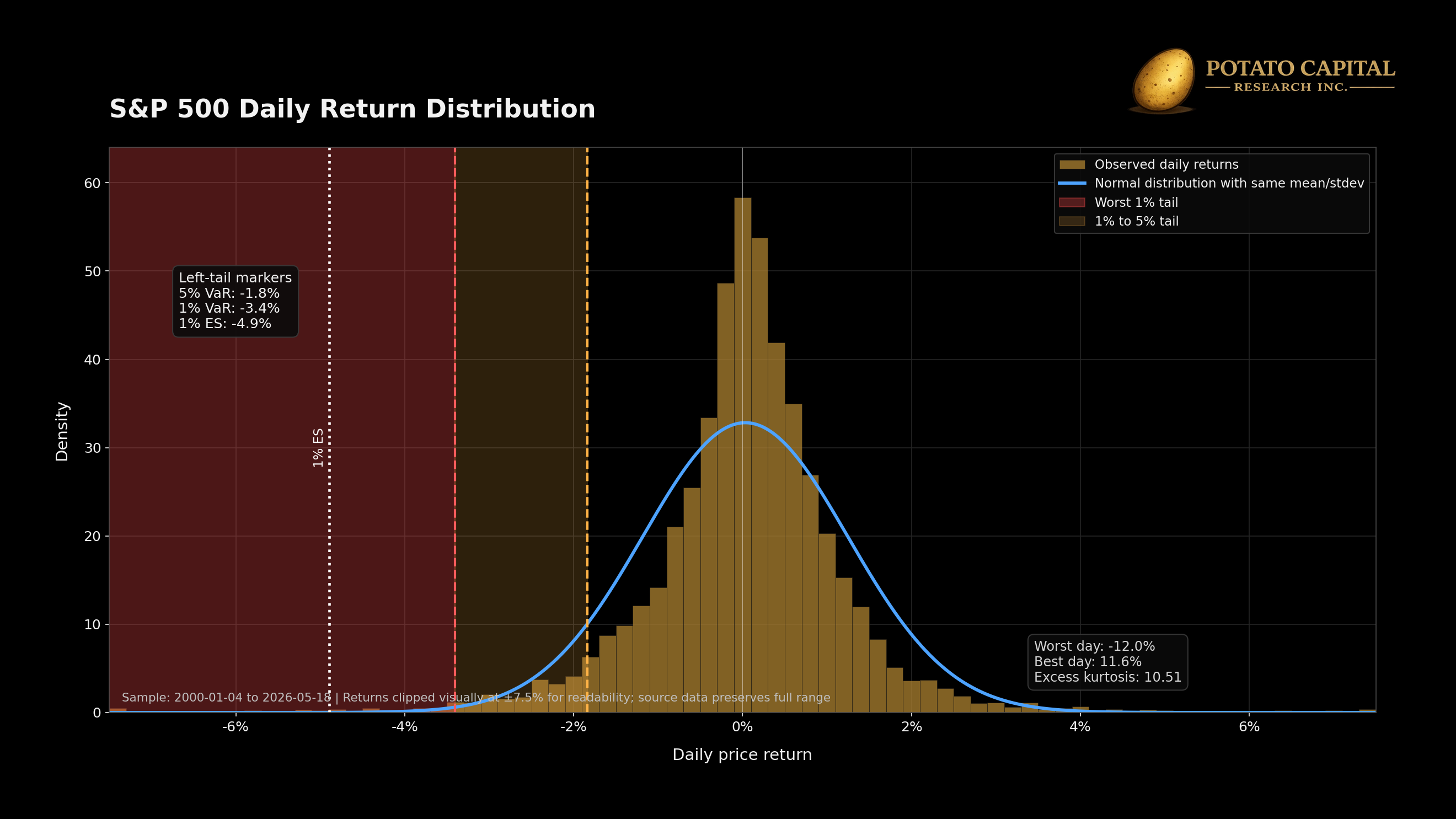
The worst daily loss was nearly 12%, and the 1% expected shortfall was -4.9% versus a 1% Value at Risk cutoff of -3.4%. The cutoff tells us where the bad tail begins. Expected shortfall tells us what investors actually lived through once that tail was breached.
The drawdown path matters because losses change the capital base. A 50% decline requires a 100% gain to recover, before considering leverage, taxes, redemptions, margin calls, or liquidity constraints. Once those frictions enter the equation, the timing of losses can matter as much as the full-period return.
Standard deviation is useful, but it treats upside and downside movement symmetrically. Expected shortfall gets closer to the portfolio question that matters in a selloff: once the bad tail is breached, how much capital is actually at risk, and does the investor still have enough liquidity and flexibility to keep operating?
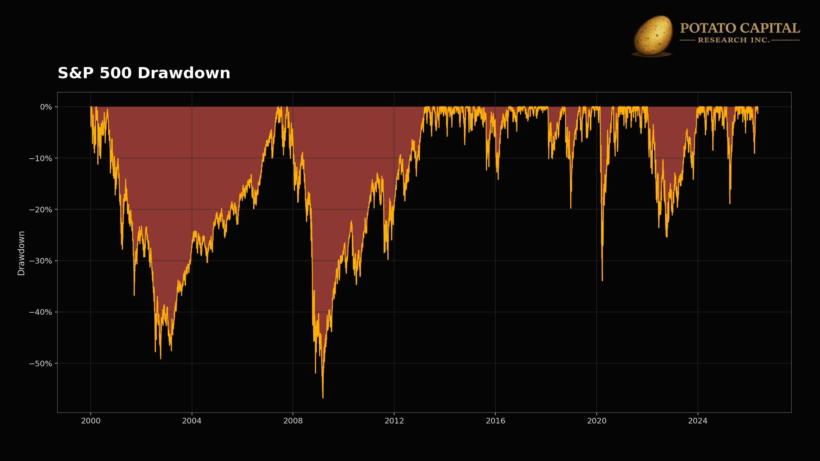
The S&P 500’s -56.8% maximum drawdown from October 2007 to March 2009 is the number that matters for survival. A portfolio cut in half needs the next cycle to do twice the work just to get back to even. Later drawdowns came from different sources: 2020 was a sudden growth shock, while 2022 was a duration and inflation repricing. Same index, different left-tail mechanisms. The long-run equity return only matters if the portfolio can live through the path required to earn it.
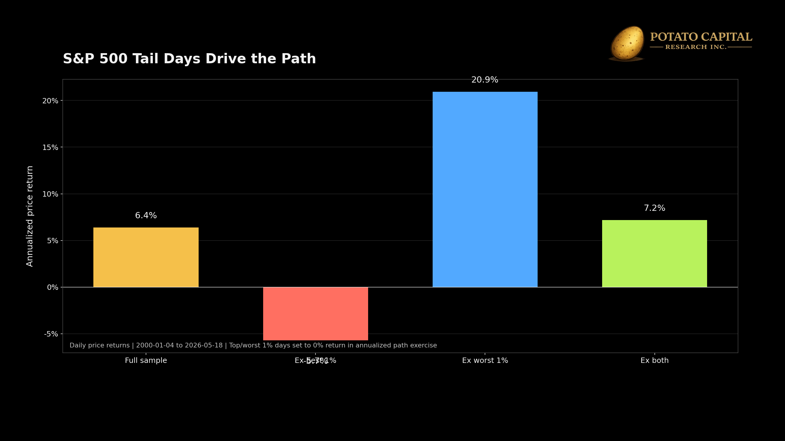
The tail-day math is just as important. From January 2000 through May 2026, the full S&P 500 daily price series annualized at 6.4%. Remove the best 1% of days and the annualized return falls to -5.7%. Remove the worst 1% of days and it rises to 20.9%. Remove both tails and the annualized return lands near 7.2%. The average return is not sitting calmly in the middle of the distribution, instead it is shaped by a small number of extreme days on both sides. The point is not that investors can reliably miss the worst days or capture only the best days; the point is that realized returns are shaped by a small number of extreme observations, which makes liquidity and staying power central to compounding.
📉 How the Left Tail Becomes Permanent
Left-tail risk becomes permanent when a mark-to-market loss forces action. For a portfolio, that can mean margin calls, redemptions, liquidity gaps, or selling because the position size no longer fits the mandate. For a company, it can mean refinancing pressure, covenant pressure, emergency equity issuance, asset sales at weak prices, or operating cuts that damage the franchise.
The balance sheet is usually where the damage shows up first. Equity investors can debate revenue, margins, and multiples for a long time, but credit shortens the timeline. A business with declining revenue and no leverage may survive long enough to recover. A similar business with near-term maturities, floating-rate debt, weak interest coverage, and poor cash conversion can lose the equity before the operating thesis has time to play out.
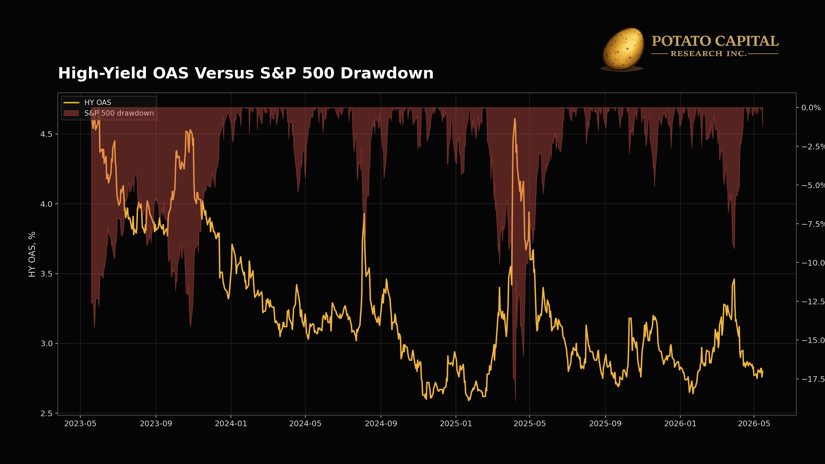
That is why credit spreads belong in a tail-risk framework. Wider spreads increase the cost of refinancing, reduce access to capital, and make equity dilution more likely for weak balance sheets. The equity market often focuses on earnings revisions first, but the permanent-impairment risk usually comes from the funding channel: debt gets harder to roll, liquidity gets more expensive, and shareholders absorb the cost.
Duration is another left-tail channel. Long-duration equities and long-duration bonds both rely heavily on cash flows far in the future. When discount rates rise, the present value of those future cash flows falls. The 2020 to 2023 bond drawdown mattered because Treasuries generated a severe mark-to-market loss without credit impairment. Inflation and rate repricing were enough.
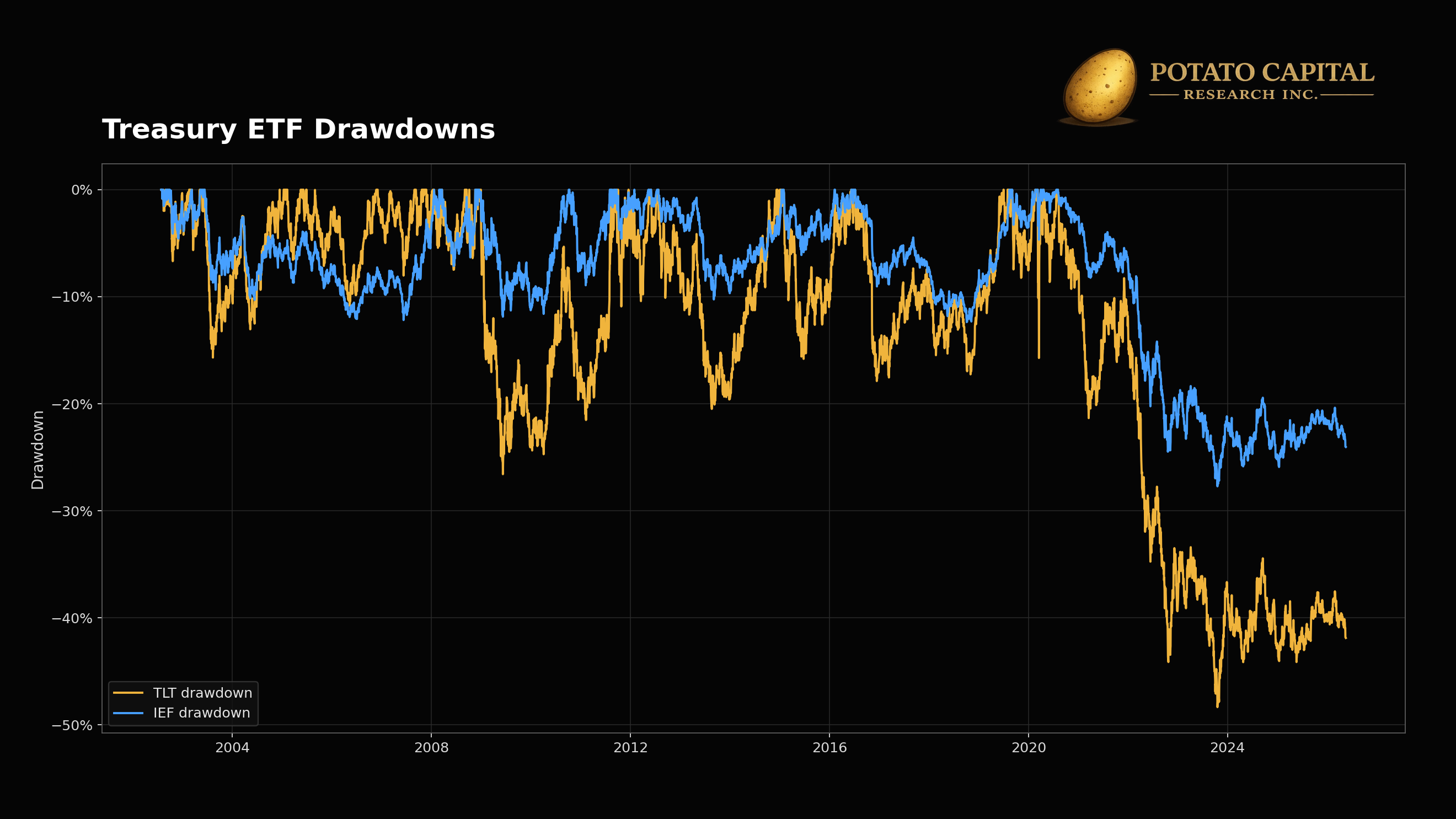
TLT’s nearly 50% drawdown is the cleanest warning from the rates side. Investors often treat duration as portfolio ballast, but the hedge works best when the shock is recessionary disinflation. In an inflation or term-premium shock, duration can become a drawdown source. IEF’s smaller decline shows the same mechanism with less maturity exposure: shorter duration reduced the damage, but did not remove it.
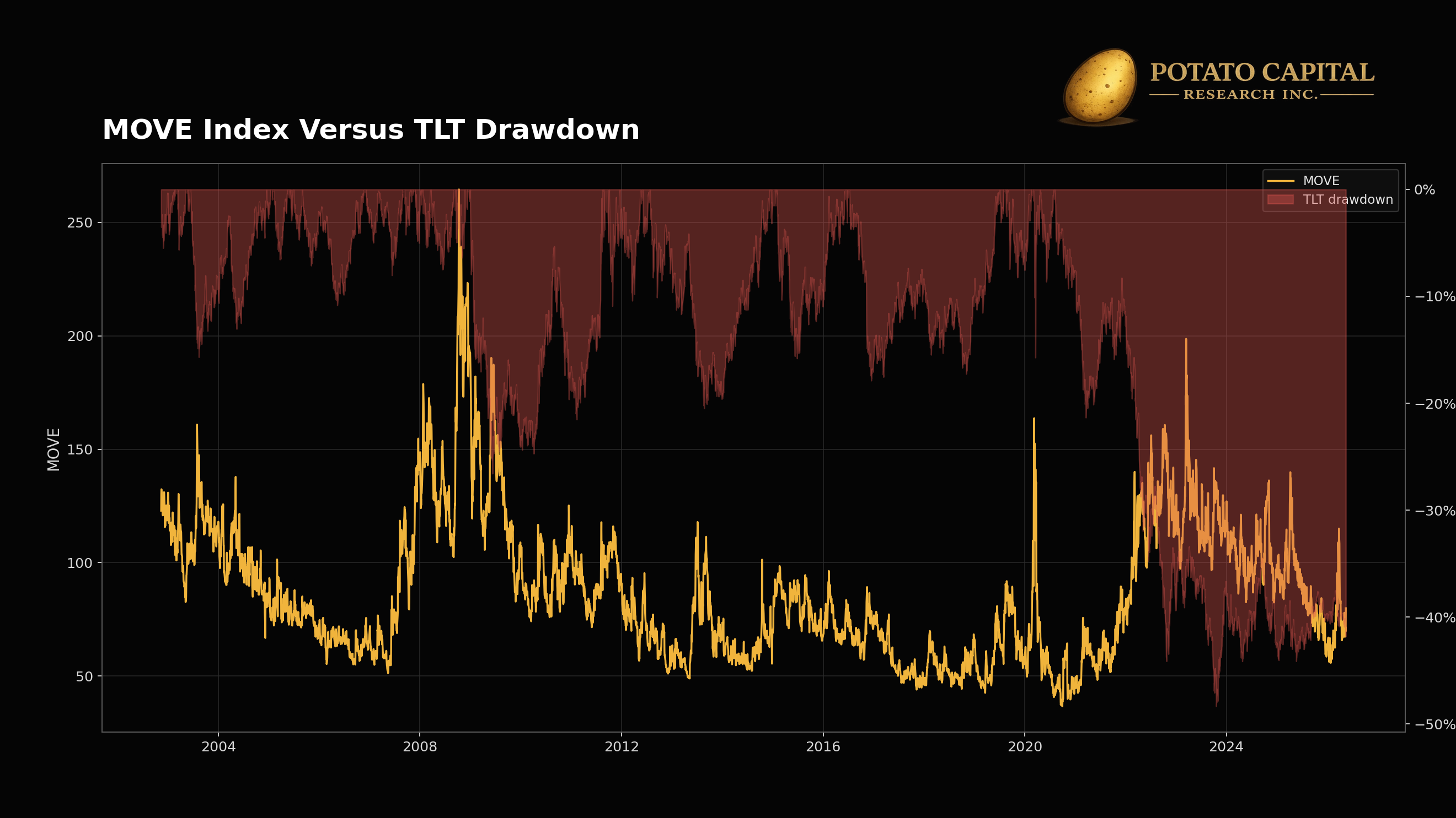
Rates volatility explains why the duration tail can move quickly. When MOVE rises, long-duration assets are being repriced through the discount-rate channel, not the default channel, which distinctively matters for portfolio construction. A Treasury-heavy hedge can still fail if the shock is higher real rates, higher inflation risk, or higher term premium rather than falling growth expectations.
Leverage adds another layer. Margin debt does not cause every selloff, but it can make a correction more fragile once volatility rises and collateral values fall. FINRA customer margin debit balances reached $1.304 trillion in April 2026, the highest level in the FINRA series used here. Debit balances were up 53.3% year over year, while net debit balances sat near the January high.
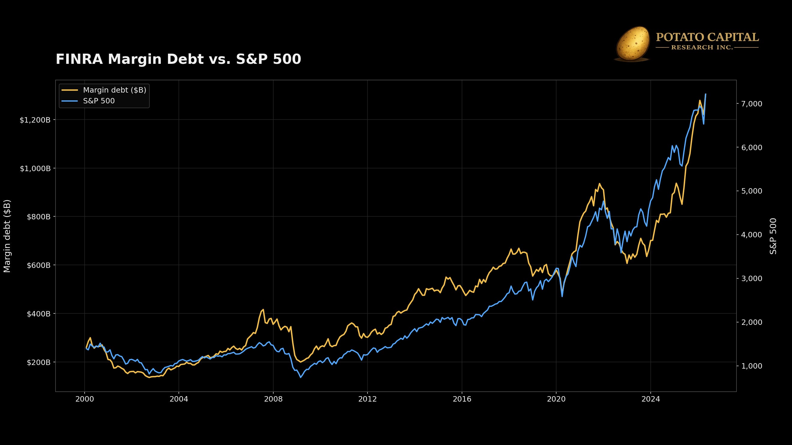
The point is vulnerability, not timing. Elevated margin debt means more forced-selling fuel if volatility, credit spreads, and equity drawdowns begin moving together. That is how a normal correction becomes a liquidation problem: collateral falls, leverage has to come down, liquidity thins, and investors sell what they can rather than what they want.
The practical monitoring list becomes leverage, refinancing risk, liquidity, margin resilience, valuation duration, accounting quality, policy exposure, and forced-selling pressure. Those risks become dangerous when they cluster - spreads widen, cash conversion weakens, liquidity thins, and position sizes built for calm markets start to break.
📈 Right Tail Optionality is not the Same as Speculation
Right tail optionality is the part of the distribution where a small number of outcomes can drive a disproportionate share of returns. In equities, the payoff usually needs more than revenue growth. The better setups have a mechanism that lets incremental revenue convert into cash flow at an improving rate through operating leverage, pricing power, capital-light scale, high incremental returns, or a long reinvestment runway.
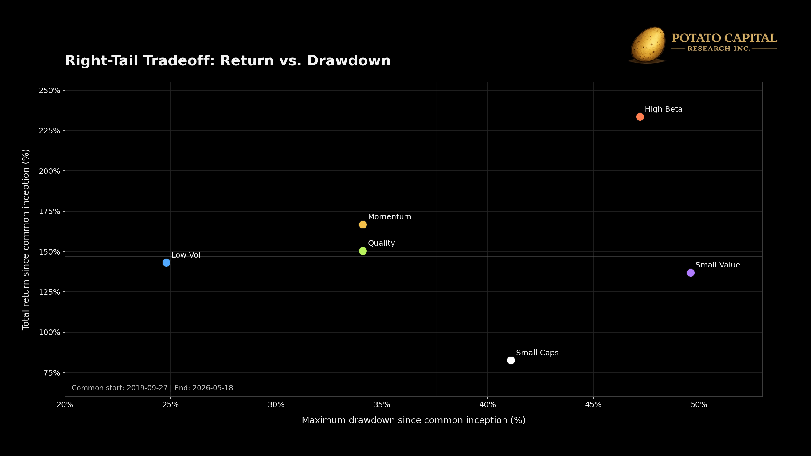
The factor evidence shows the market version of the tradeoff. Since September 2019, high beta delivered the strongest return in the group, but it also came with a much deeper drawdown than low volatility or quality. That is the basic bargain with right-tail exposure. The upside can be real, but the path is usually less forgiving. Position size has to account for the drawdown profile, not only the upside case.
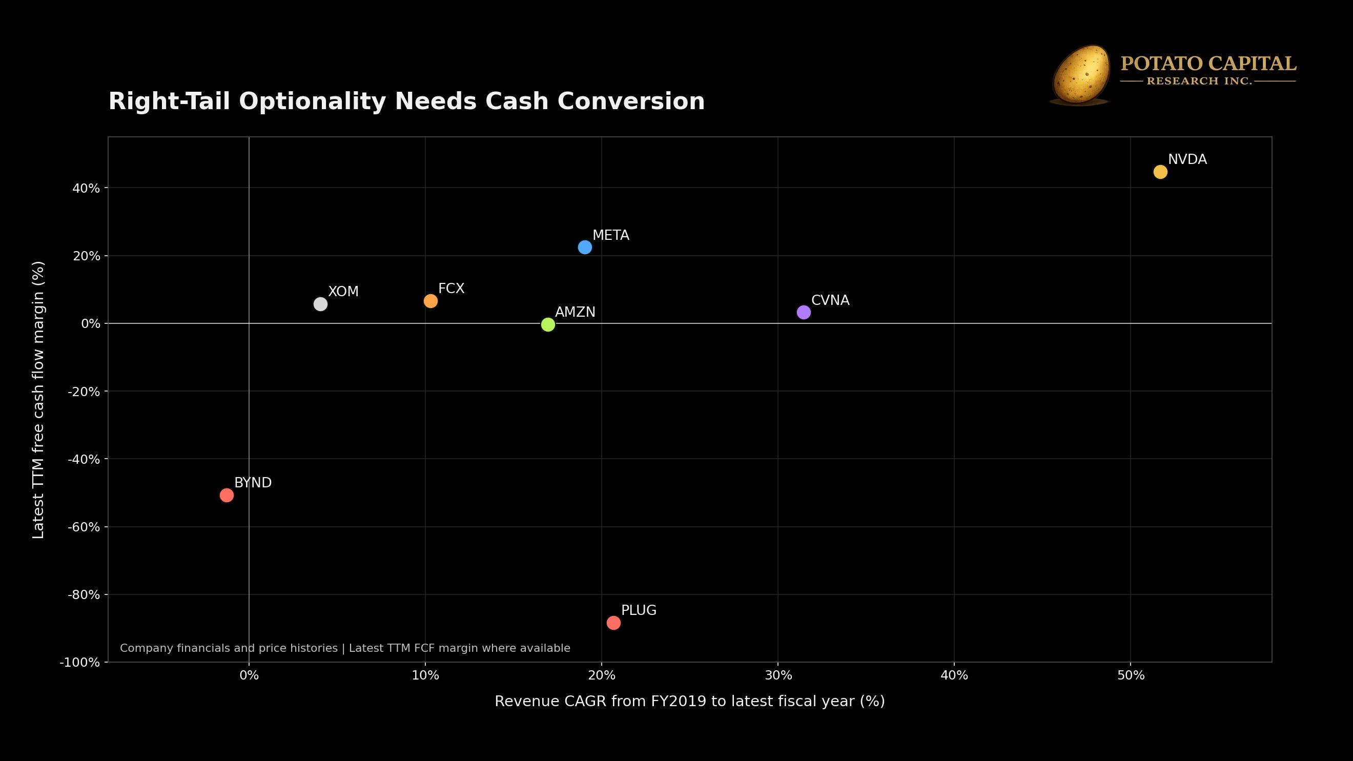
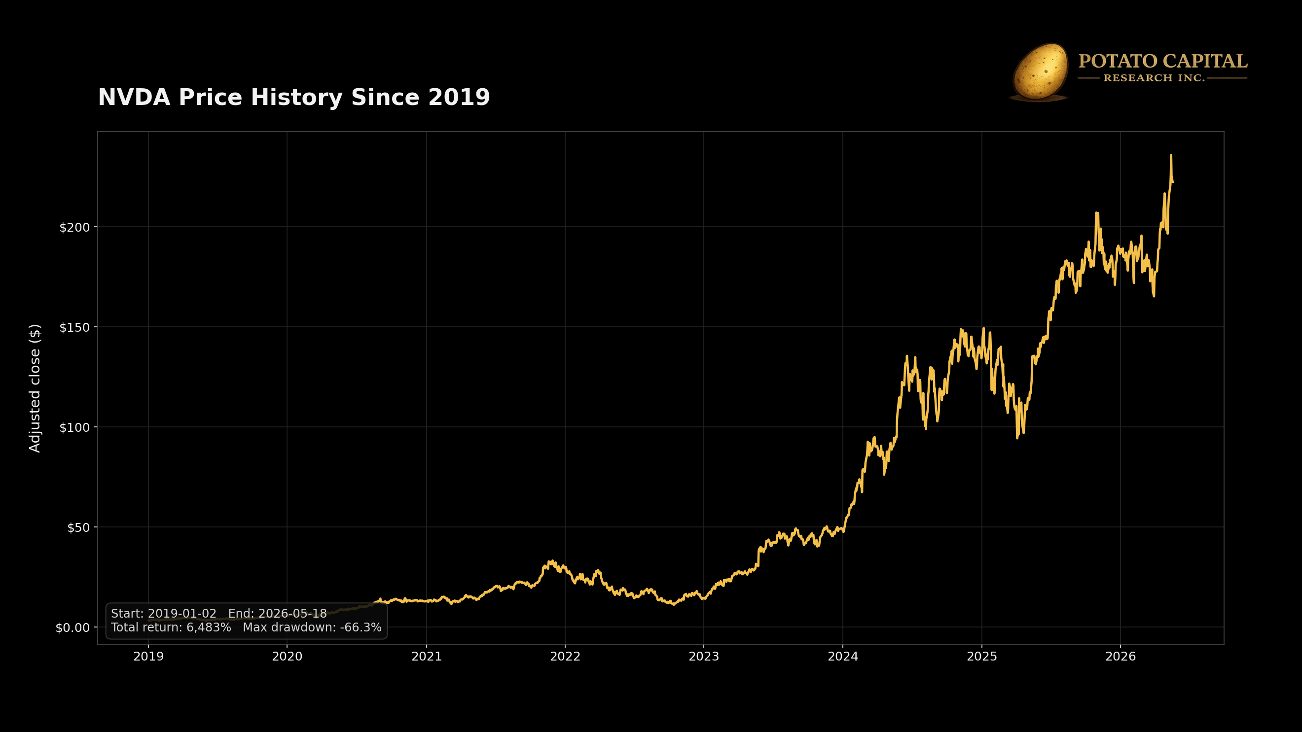
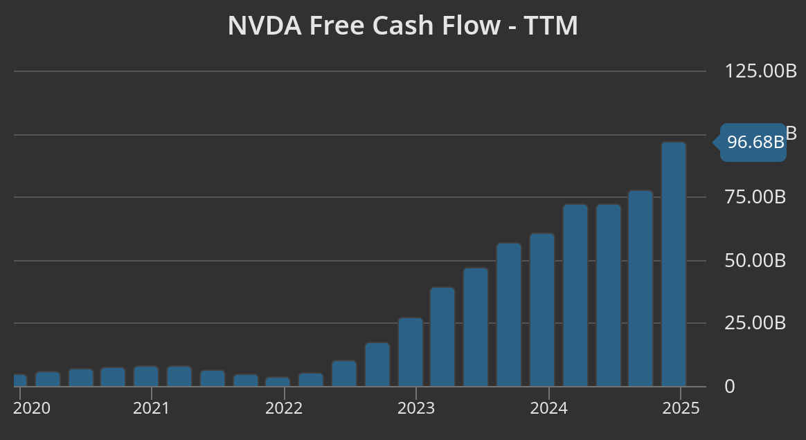
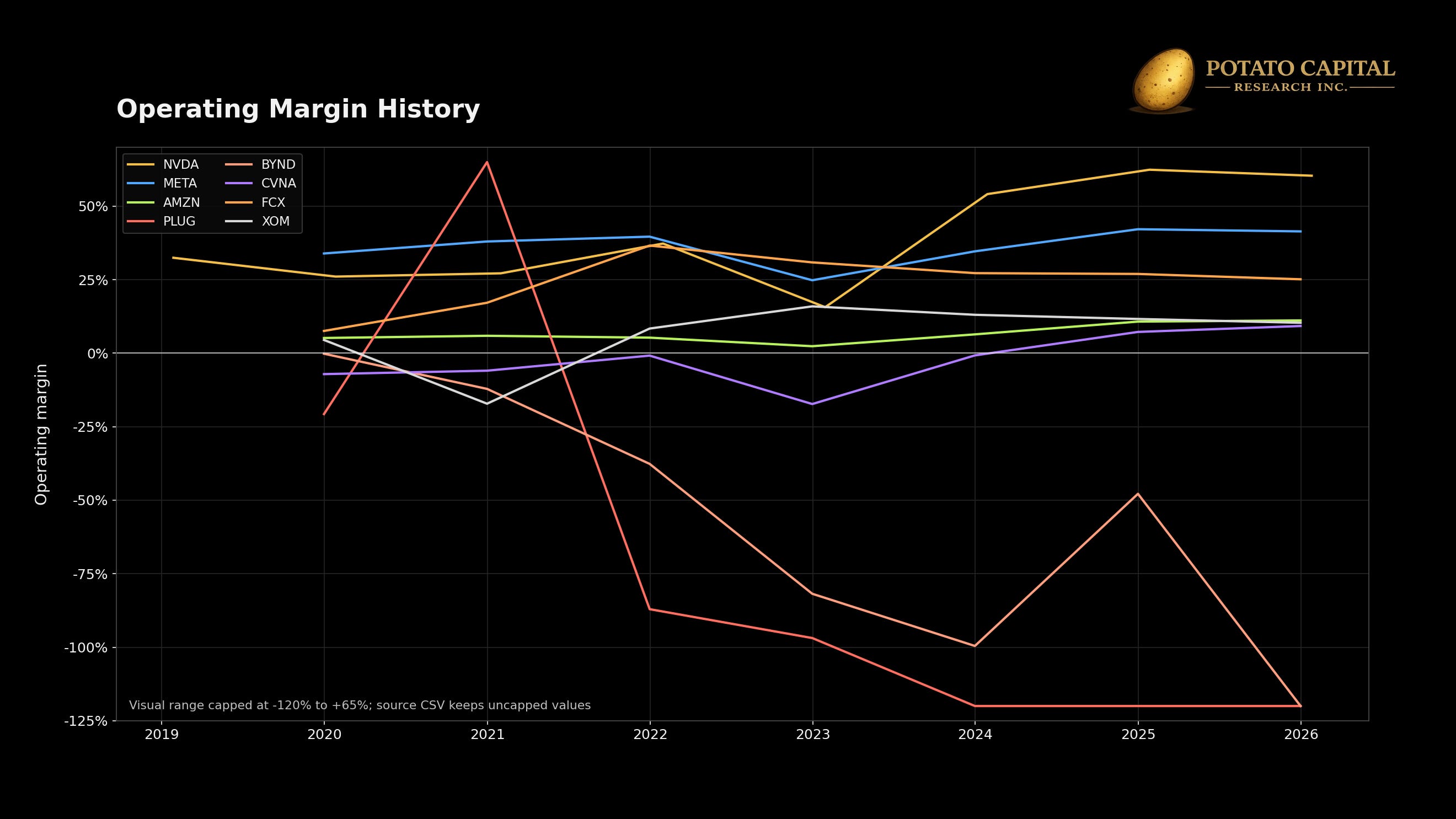
Single-name data sharpens the point. The right tail becomes much higher quality when the upside is backed by cash conversion, margin expansion, and limited dilution. NVDA is the cleanest example in our company set. From fiscal 2019 to the latest fiscal year, revenue compounded at 51.7%, latest TTM free cash flow margin reached 44.8%, and the stock returned roughly 5100%. Diluted share count also fell slightly over the period. That combination matters because NVDA growth translated into cash flow, and the upside accrued to shareholders rather than being offset by dilution.
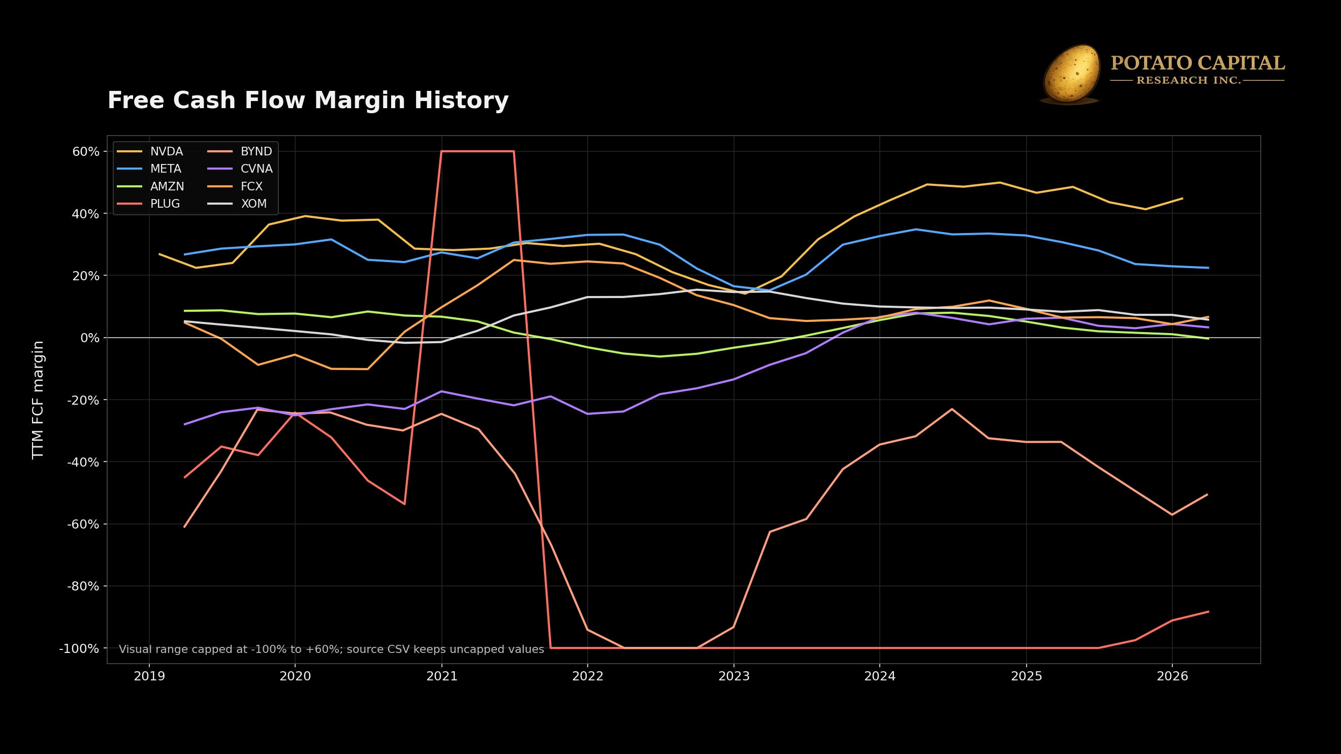
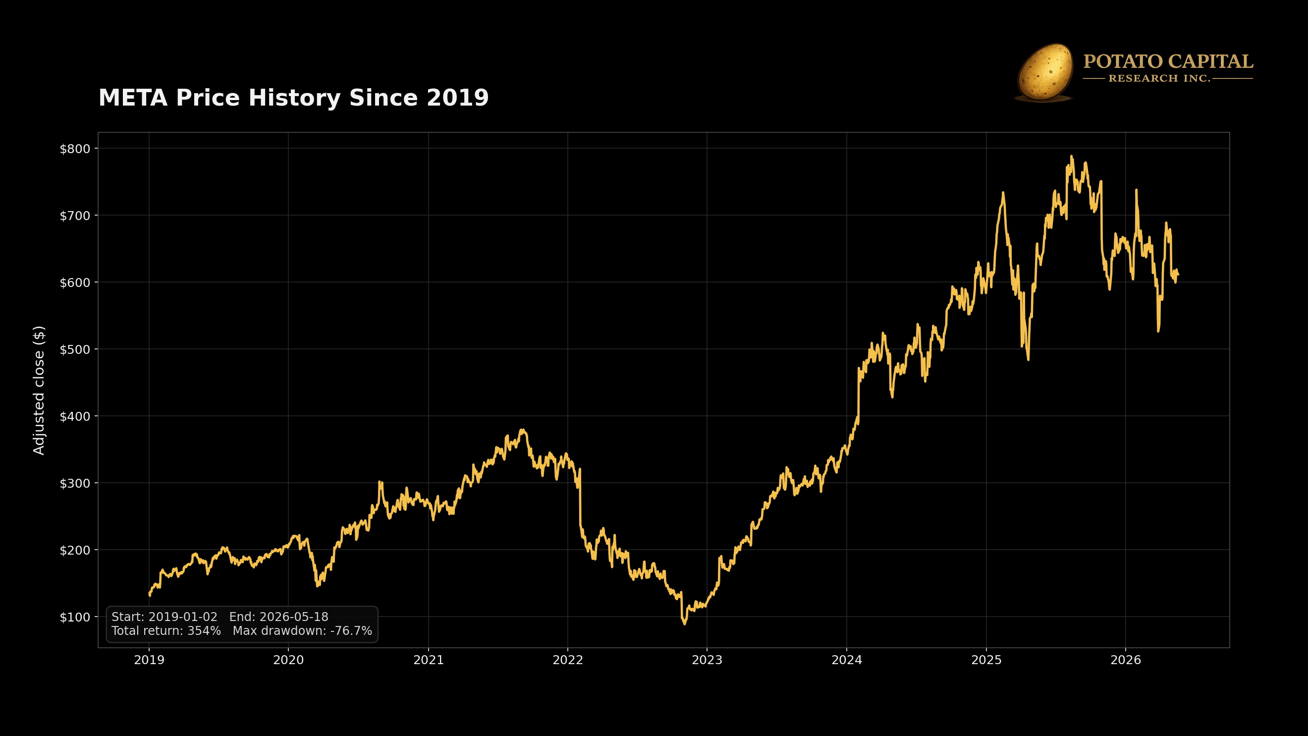
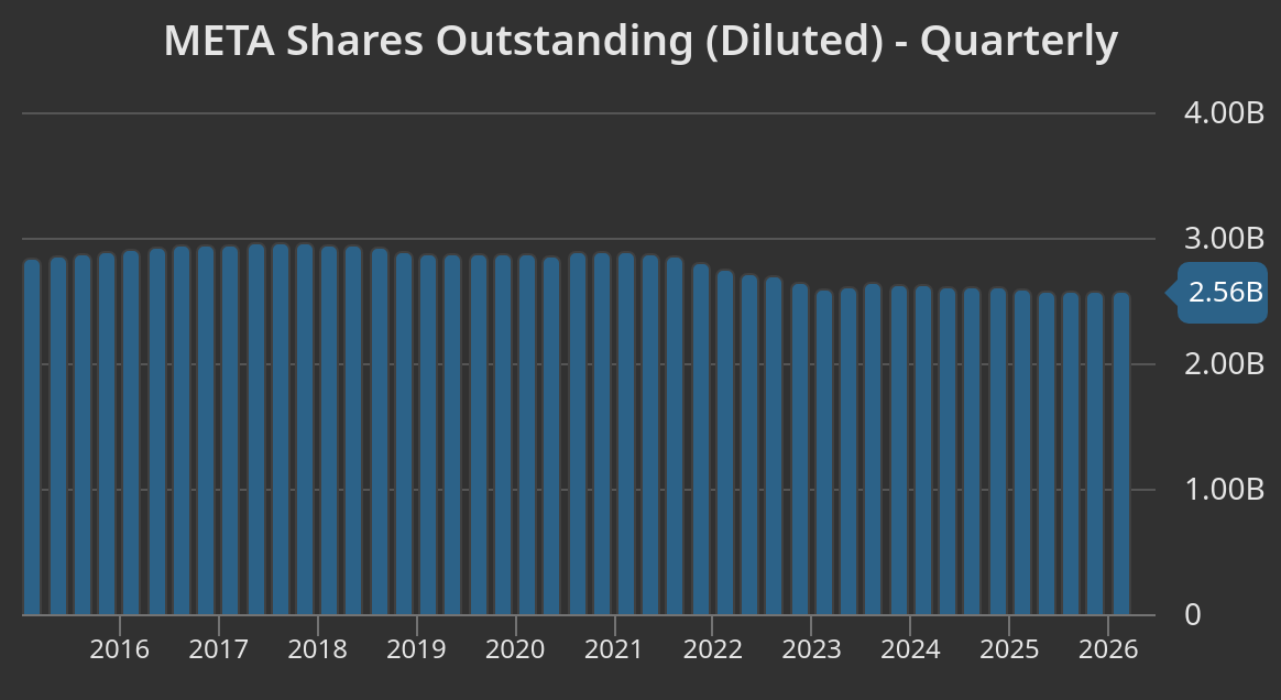
META shows a different version of the same idea. Revenue compounded at 19.0%, latest TTM free cash flow margin was 22.5%, and diluted share count fell 10.5%. The stock path was still painful, with a -76.7% maximum drawdown, but the business kept generating cash and reducing dilution risk. The right tail came from operating leverage and capital discipline after the market had already punished the stock.
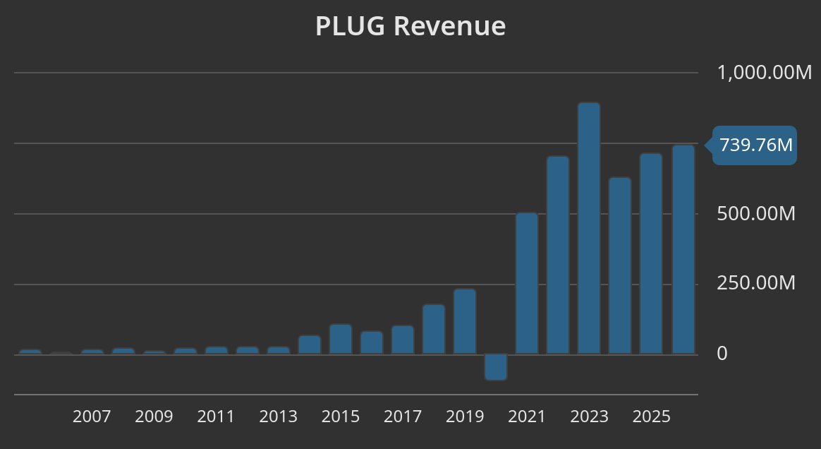
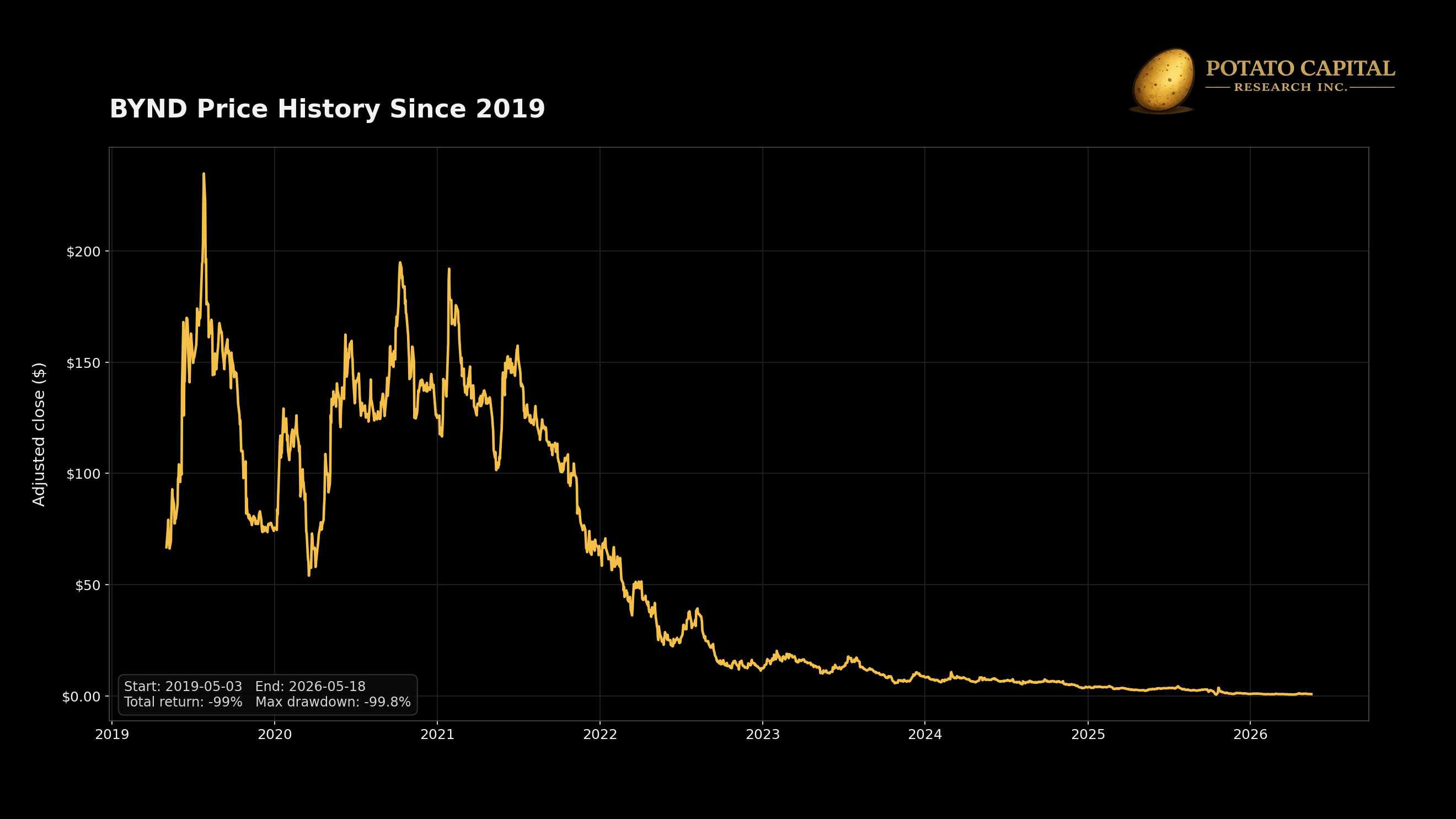
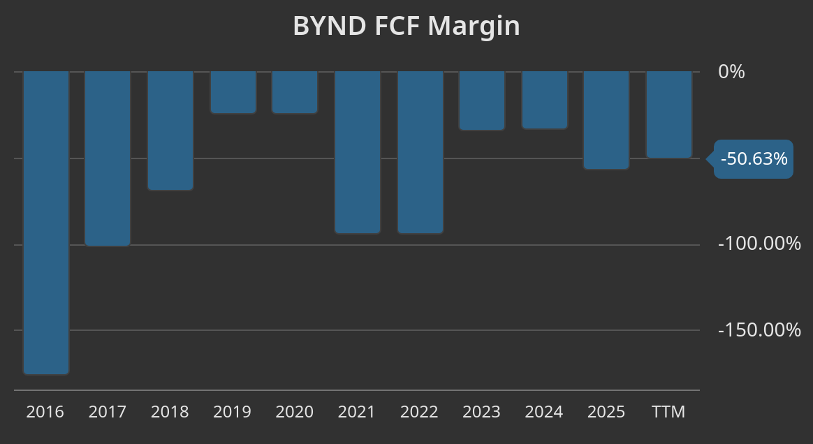
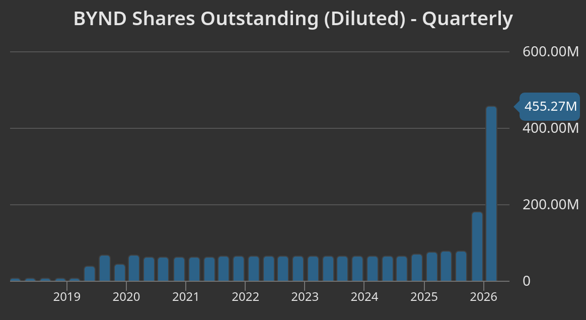
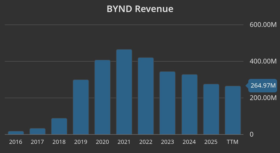
PLUG and BYND show why upside language needs proof. PLUG compounded revenue at 20.7%, but latest TTM free cash flow margin was -88.3%, the stock suffered a -99.0% maximum drawdown, and diluted share count increased more than 380%. BYND had a similar equity outcome with weaker growth: revenue declined slightly on a compound basis, latest TTM free cash flow margin was -50.6%, the stock fell 99.5% from the September 2019 reference point, and diluted share count increased roughly 328%. The economics did not support the optionality.
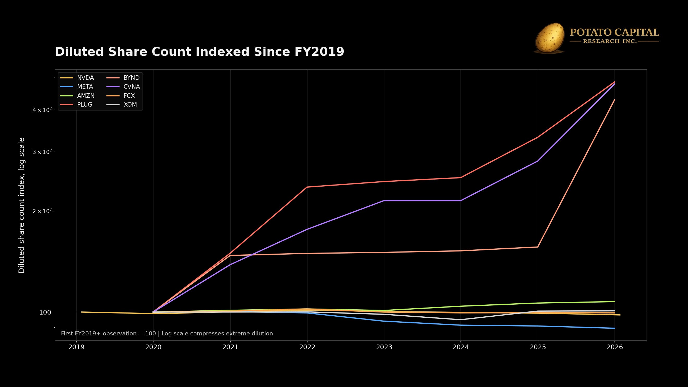
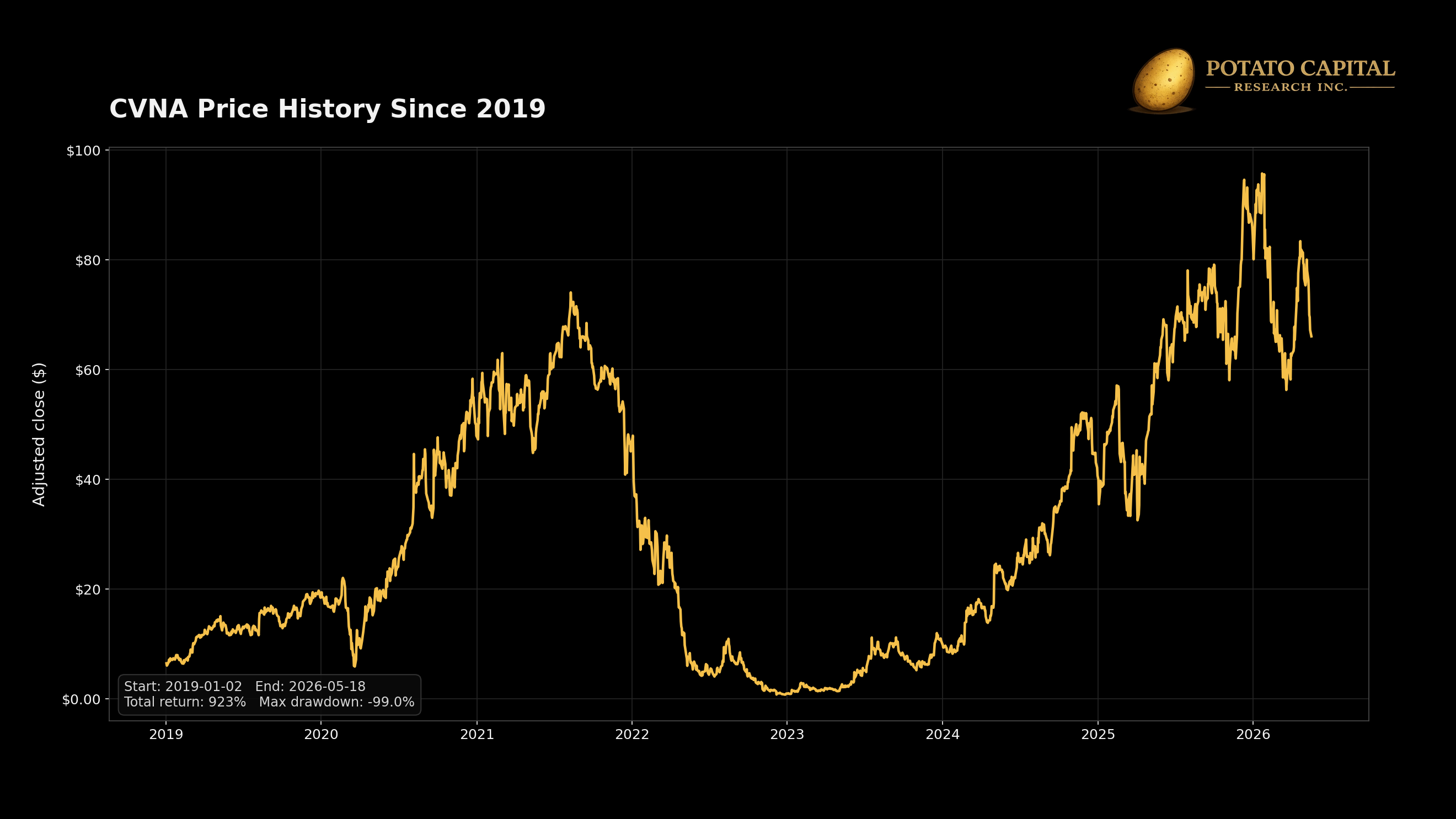
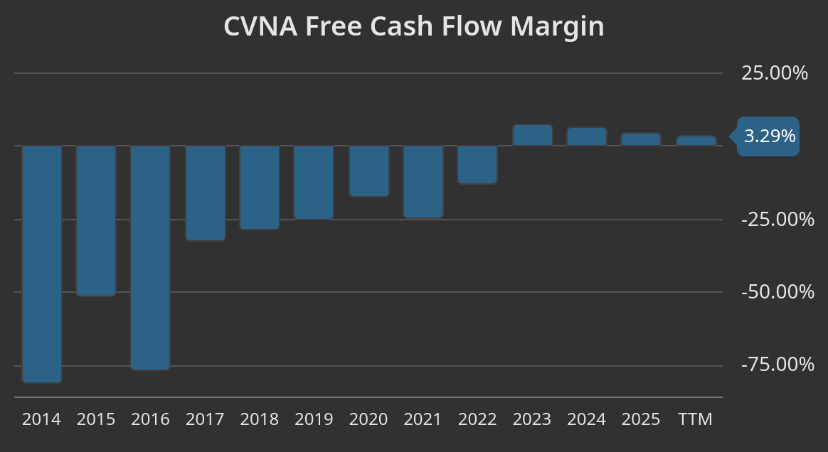
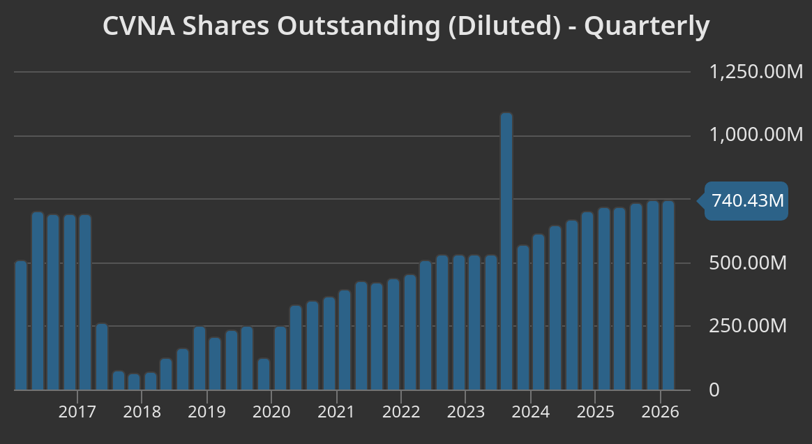
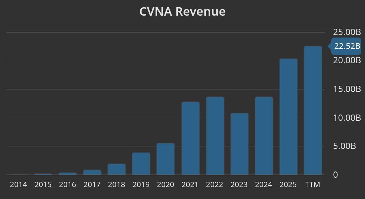
CVNA is the useful middle case. The equity delivered a large return from the September 2019 reference point, but the path was extreme. Revenue compounded at 31.4%, latest TTM free cash flow margin was positive at 3.3%, and the stock returned roughly 400%. The cost was a -99.0% maximum drawdown and a roughly 377% increase in diluted shares. That is distressed equity optionality: the payoff can be large, but the position can nearly disappear before the recovery shows up.
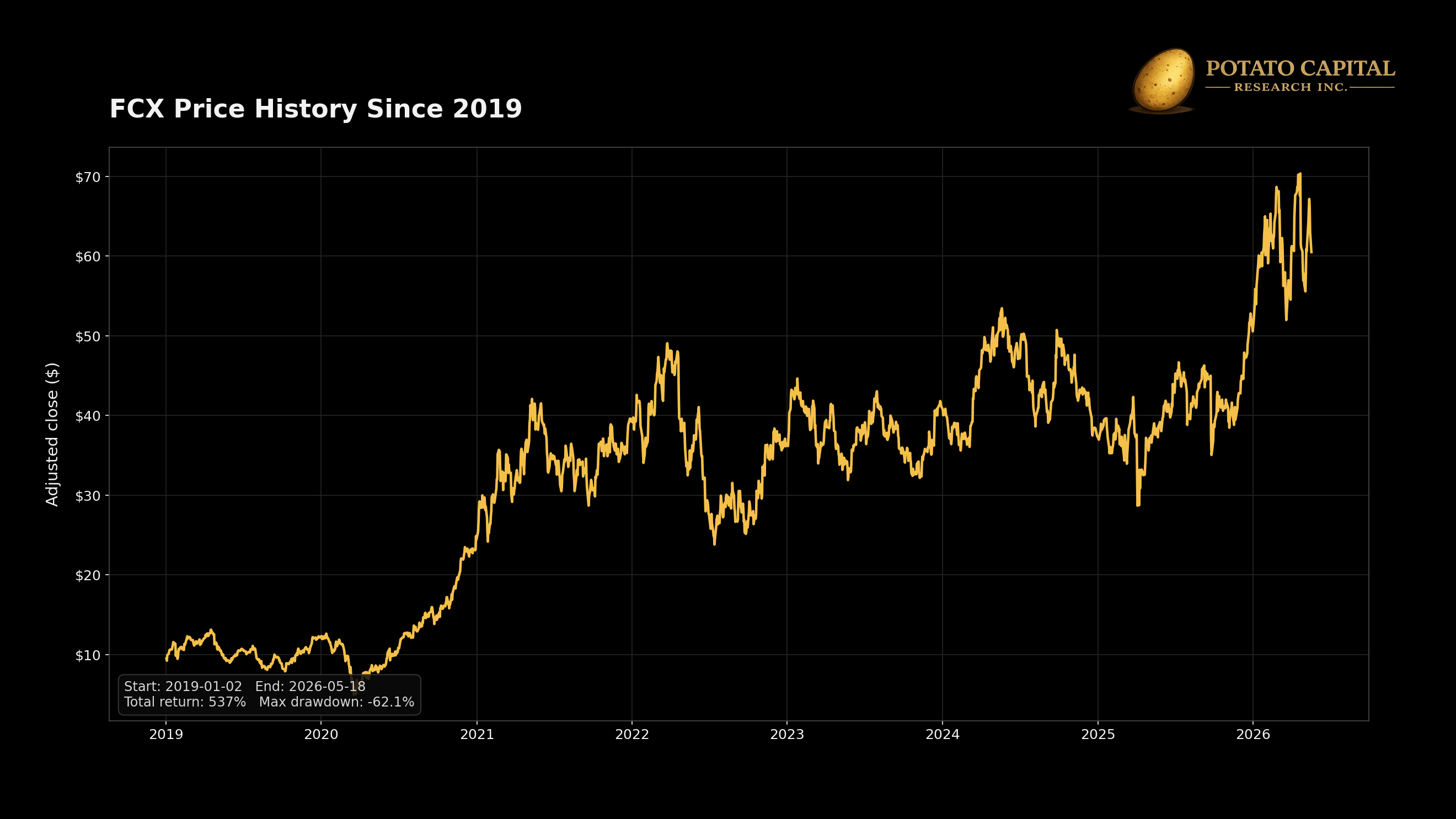
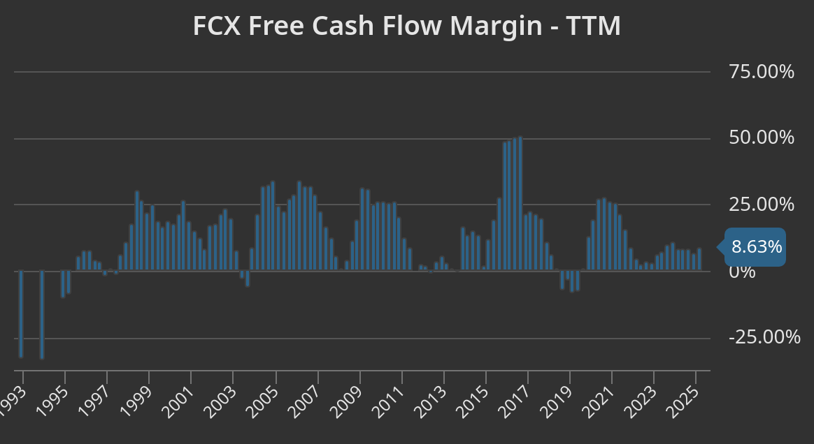
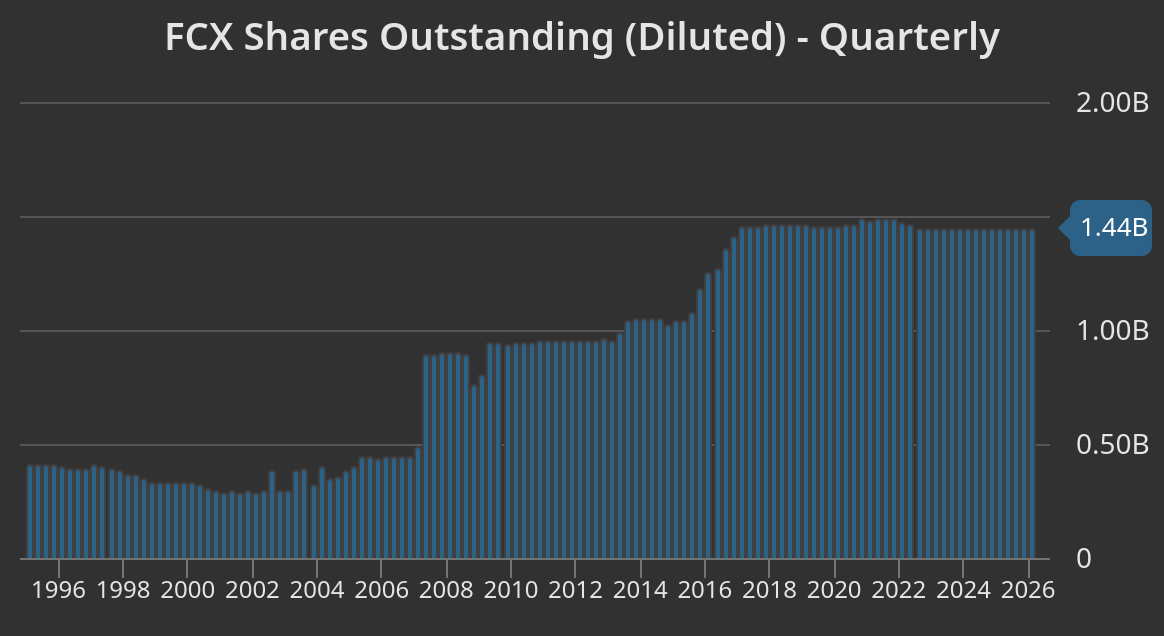
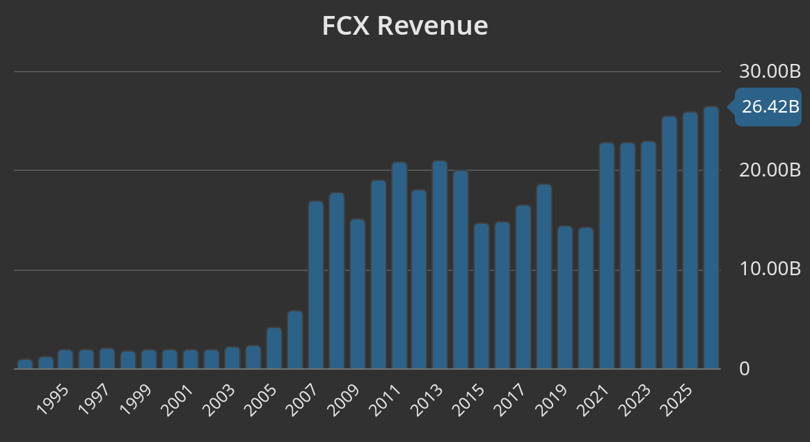
FCX adds the commodity version. Revenue compounded at 10.3%, latest TTM free cash flow margin was 6.6%, and the stock returned roughly 575% from the same reference point. The upside did not require software-like margins or secular volume growth. It came from cyclical operating leverage and commodity exposure. The tradeoff was still material, with a -60.6% maximum drawdown over the period.
The evidence separates right tail exposure into different categories. NVDA and META were operating leverage and cash-flow conversion. FCX was commodity torque. CVNA was distressed recovery with a brutal path. PLUG and BYND were upside stories without durable cash economics or dilution control.
That distinction matters for sizing. Growth with improving free cash flow can graduate into core exposure. Commodity torque belongs in a cyclical sleeve. Distressed recovery belongs in an option-sized sleeve. Revenue growth with deeply negative free cash flow and heavy dilution needs a much higher burden of proof.
Chart Dump (Company evidence: when optionality becomes economics):
💰 Valuation Needs a Distribution, Not Just a Target
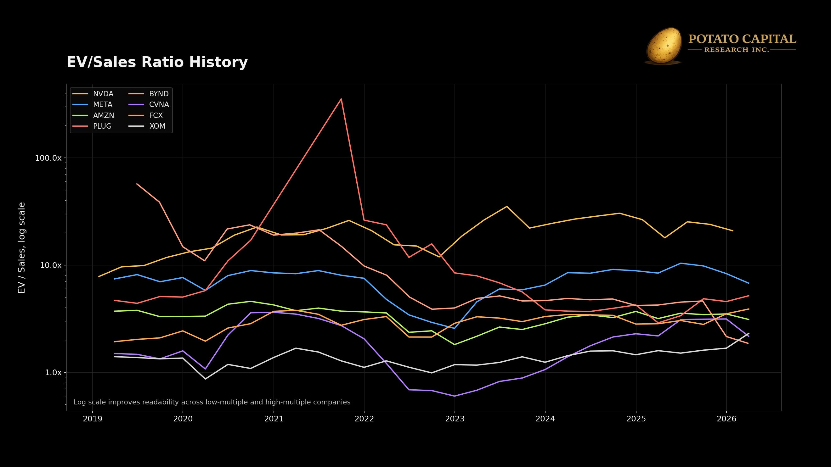
Single-point valuation is useful for discipline, but it can hide the part of the distribution that matters most. A multiple tells us what the market is paying today, but does not tell us whether the business has enough cash conversion, margin runway, balance-sheet strength, or dilution control to justify the path embedded in that multiple.
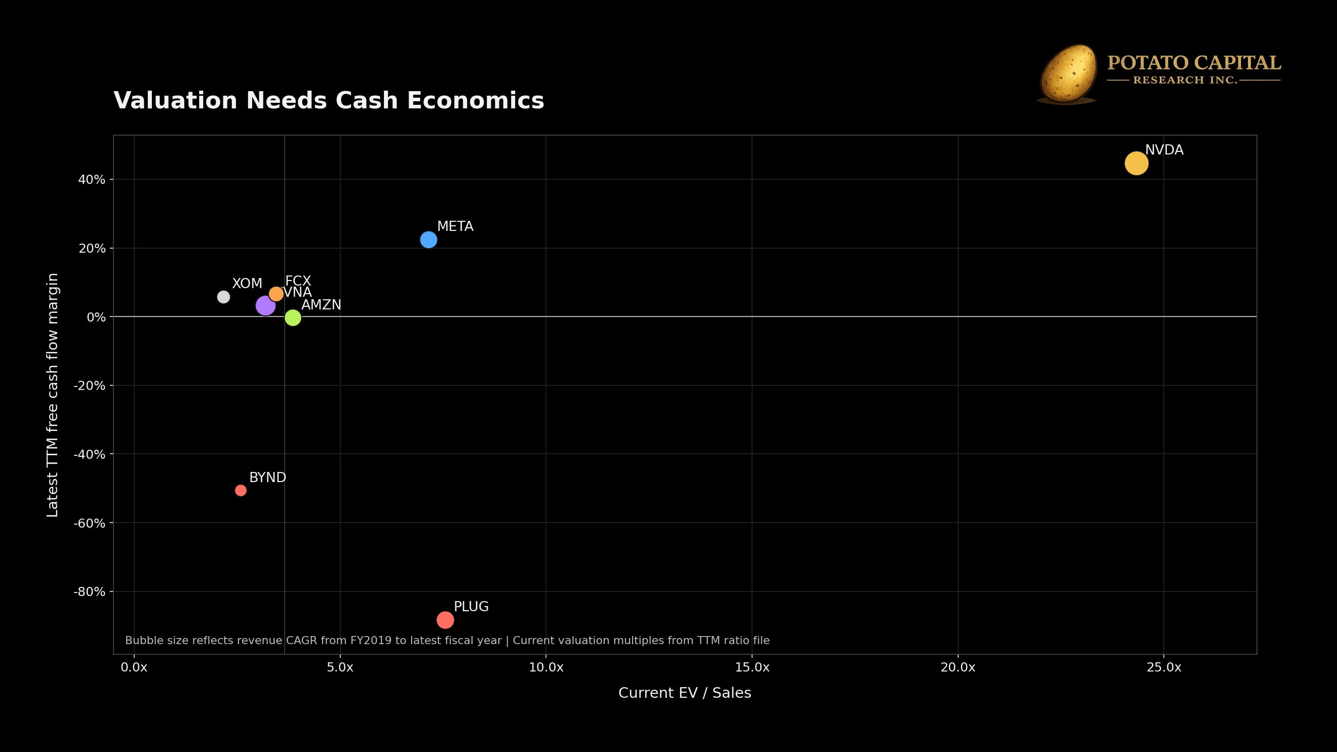
Our company set shows why the label “cheap” or “expensive” is incomplete without the economics behind it. NVDA sits at the expensive end of current TTM EV/sales, but it also has the strongest free cash flow margin in the group and the highest revenue CAGR since fiscal 2019. PLUG and BYND sit much lower on EV/sales, but both have deeply negative free cash flow margins and heavy dilution. The valuation question is not the multiple in isolation, but whether the business can convert the implied expectations into cash flow that accrues to shareholders.
NVDA currently screens expensive on simple current TTM multiples - roughly 24.3x EV/sales and 54.9x P/FCF. That valuation would be harder to defend if the company were only showing revenue growth. The support comes from our full evidence set: 51.7% revenue CAGR from fiscal 2019 to the latest fiscal year, 44.8% latest TTM free cash flow margin, and a lower diluted share count. In valuation terms, the bull case is not only AI growth in the abstract, but growth converting into high-margin free cash flow without meaningful dilution.
PLUG sits on the other side of that evidence. Revenue compounded at 20.7% from fiscal 2019 to the latest fiscal year, but latest TTM free cash flow margin was -88.3%, diluted share count rose more than 380%, and the stock suffered a -99% maximum drawdown from the September 2019 reference point. A low or compressed multiple does not solve poor unit economics. If growth requires repeated external capital and shareholder dilution, the equity can still be expensive on a probability-adjusted basis.
CVNA is the path-dependency case: the stock returned roughly 400% from the September 2019 reference point, but the path included a -99% maximum drawdown and roughly 377% diluted share count growth. Latest TTM free cash flow margin is now positive at 3.3%, while current valuation remains demanding at roughly 93.1x P/FCF and 30.6x EV/EBITDA. That is why valuation needs more than a target price. The payoff was legitimate, but the interim path looked closer to distressed optionality than a normal compounder.
FCX and XOM show why the macro regime also belongs inside valuation. FCX returned roughly 575% from the September 2019 reference point with a 10.3% revenue CAGR and 6.6% latest TTM free cash flow margin. XOM returned roughly 204% with a 4.0% revenue CAGR and 5.8% latest TTM free cash flow margin. Those outcomes were driven less by secular growth and more by commodity-cycle exposure, capital discipline, and the starting point of the cycle. A static terminal multiple would miss how quickly the same business can move between cheap and rich depending on the commodity backdrop.
The valuation process should therefore be distributional. The base case should reflect the central evidence after reconciling operating data, balance-sheet risk, macro exposure, and market expectations. The bull case should identify the mechanism that creates upside: margin expansion, reinvestment returns, pricing power, lower capital intensity, commodity torque, or an asset monetization path. The bear case should identify the mechanism of impairment: refinancing pressure, margin collapse, dilution, multiple compression, or permanent revenue loss.
Reverse DCF is a useful tool because it turns the current price into an expectations test. A high-multiple stock can still work if the implied growth, margin, and reinvestment path is below what the business can actually deliver. A low-multiple stock can still be expensive if the market is correctly pricing credit stress, fading earnings power, poor cash conversion, or dilution risk.
Practically speaking, if a modest change in margin, discount rate, terminal multiple, or share count materially changes fair value, the stock owns a valuation tail. Scenario weights should move only when the evidence changes.
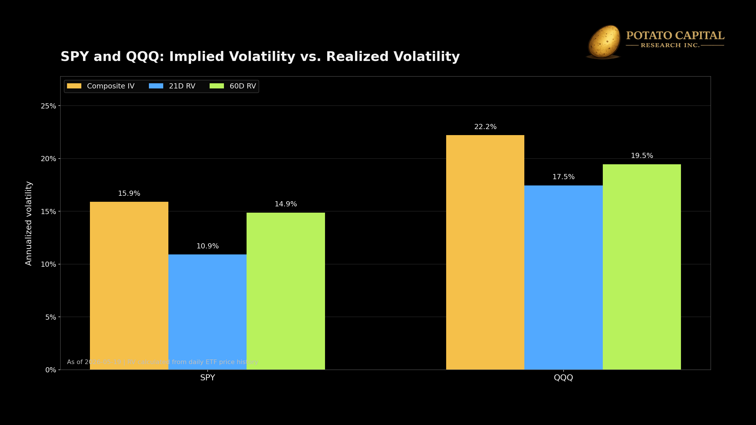
🎯 Options Markets Show what Investors are Paying to Own or Avoid Tails
Options markets turn uncertainty into prices. Implied volatility shows what investors are paying for movement. Skew shows where the demand for convexity sits. Term structure shows whether volatility risk is concentrated near term or being priced further out on the curve.
The current setup shows priced risk without the shape of a full stress regime. SPY composite implied volatility was 15.89% versus 21-day realized volatility of 10.90%, leaving a 5.0 volatility-point premium. QQQ composite implied volatility was 22.21% versus 21-day realized volatility of 17.46%, leaving a 4.8 vol-point premium. On a 60-day realized-volatility basis, the premium was much narrower for SPY at roughly 1.0 vol point, while QQQ still carried a 2.8 vol-point premium.
The comparison is more useful than the absolute level, SPY implied volatility sat above recent realized volatility, but its IV rank was only 31.1%. QQQ’s implied volatility was higher at 22.21%, with IV rank at 49.7% and IV percentile at 81%. The options market is assigning a wider distribution to the technology-heavy proxy, while broad index volatility remains below crisis-style pricing.
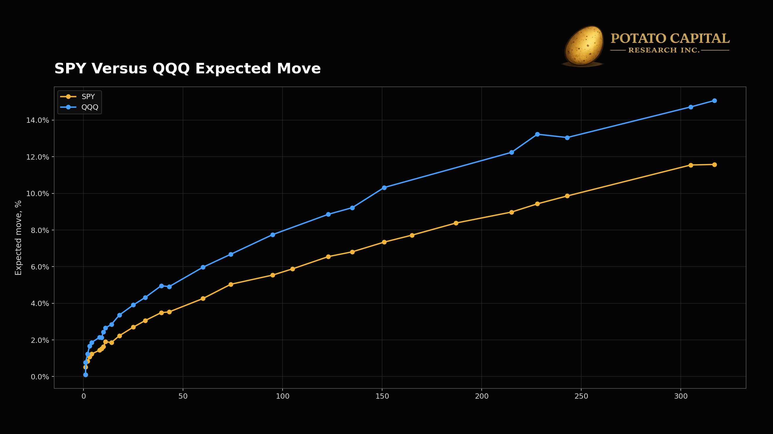
Expected move data points in a similar direction. SPY was priced for a 3.06% move over the 31-day monthly expiry and 4.26% over 60 days. QQQ was priced wider at 4.32% over 31 days and 5.97% over 60 days. Meaning investors are paying more to own or hedge QQQ path risk.
Skew shows where investors are paying for convexity. In the July 17, 2026 expiry, SPY’s approximate 25-delta put implied volatility was 19.18% versus 13.30% for the 25-delta call. QQQ’s approximate 25-delta put implied volatility was 24.90% versus 19.45% for the 25-delta call. Downside protection was richer than upside participation in both markets, with SPY showing a slightly wider 25-delta put-call skew.
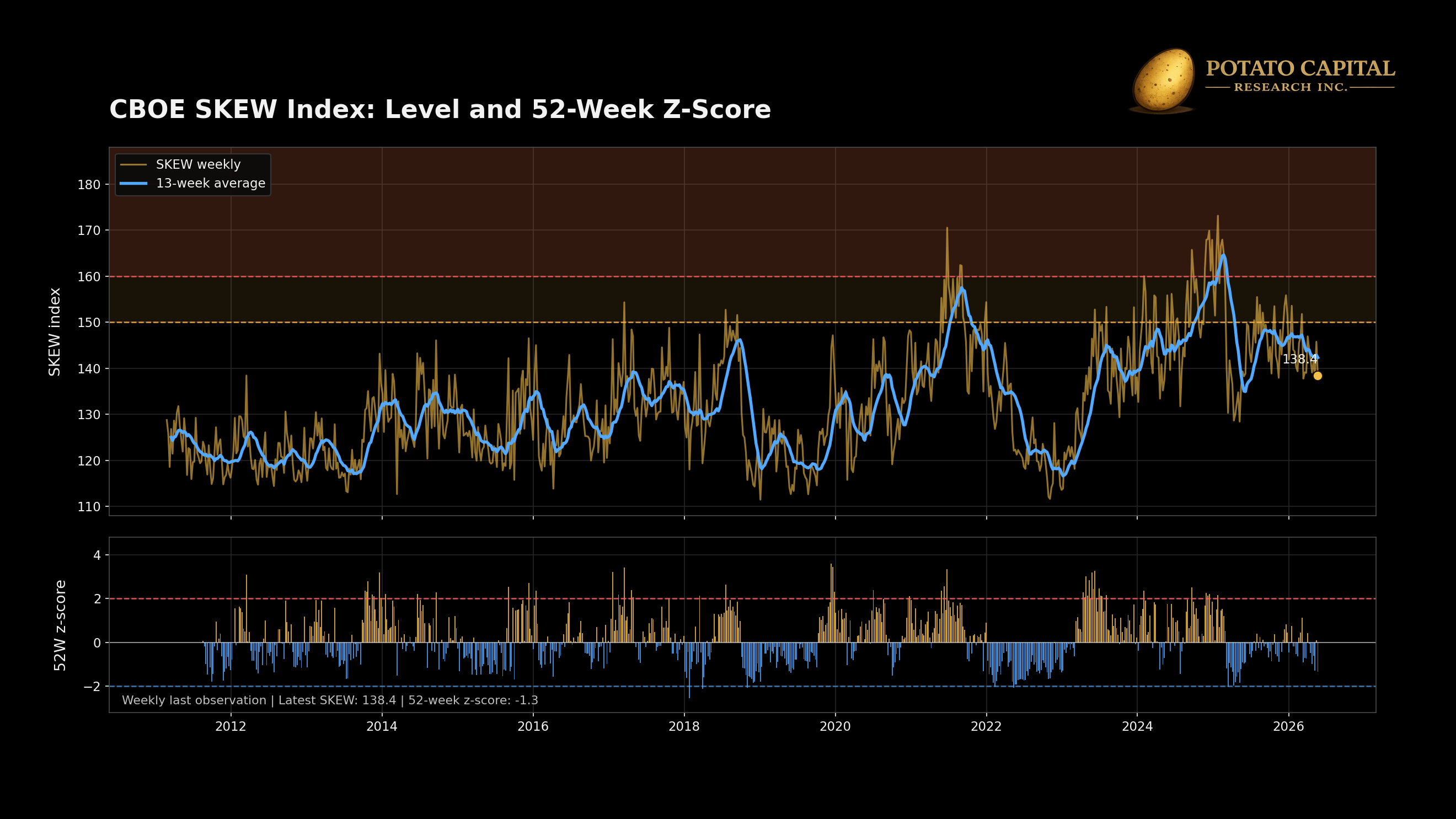
The SKEW index gives the broader index-level version of tail pricing, but it needs context. The latest reading was below its own recent 52-week norm, so it is not flashing extreme historical stress. At the same time, the options-chain still shows ( downside puts priced richer than upside calls in the July expiry. Those are different measures: historical index-level tail pricing versus current expiry-specific put-call skew.
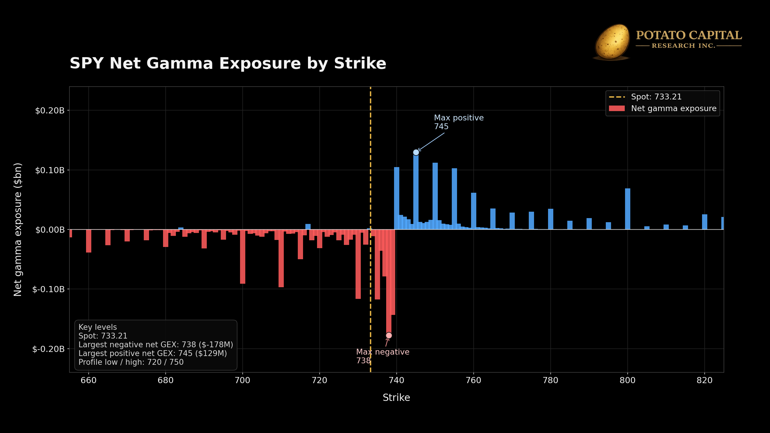
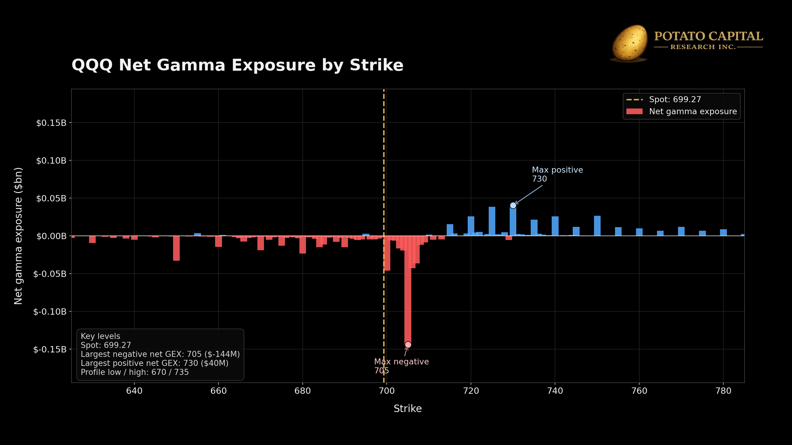
Gamma exposure adds our dealer-positioning layer. Currently, SPY’s largest negative net gamma exposure was at the 738 strike, while its largest positive net gamma exposure was at 745. QQQ’s largest negative net gamma exposure was at 705, while its largest positive net gamma exposure was at 730. These are tactical levels, not valuation evidence. Their use is path analysis: if spot trades near large negative gamma zones, hedging flows can make moves more self-reinforcing; if spot trades near large positive gamma zones, hedging flows can dampen movement. For this note, gamma helps explain how a tail move could travel through the market, while implied volatility, skew, and VIX futures explain what investors are paying for that risk.
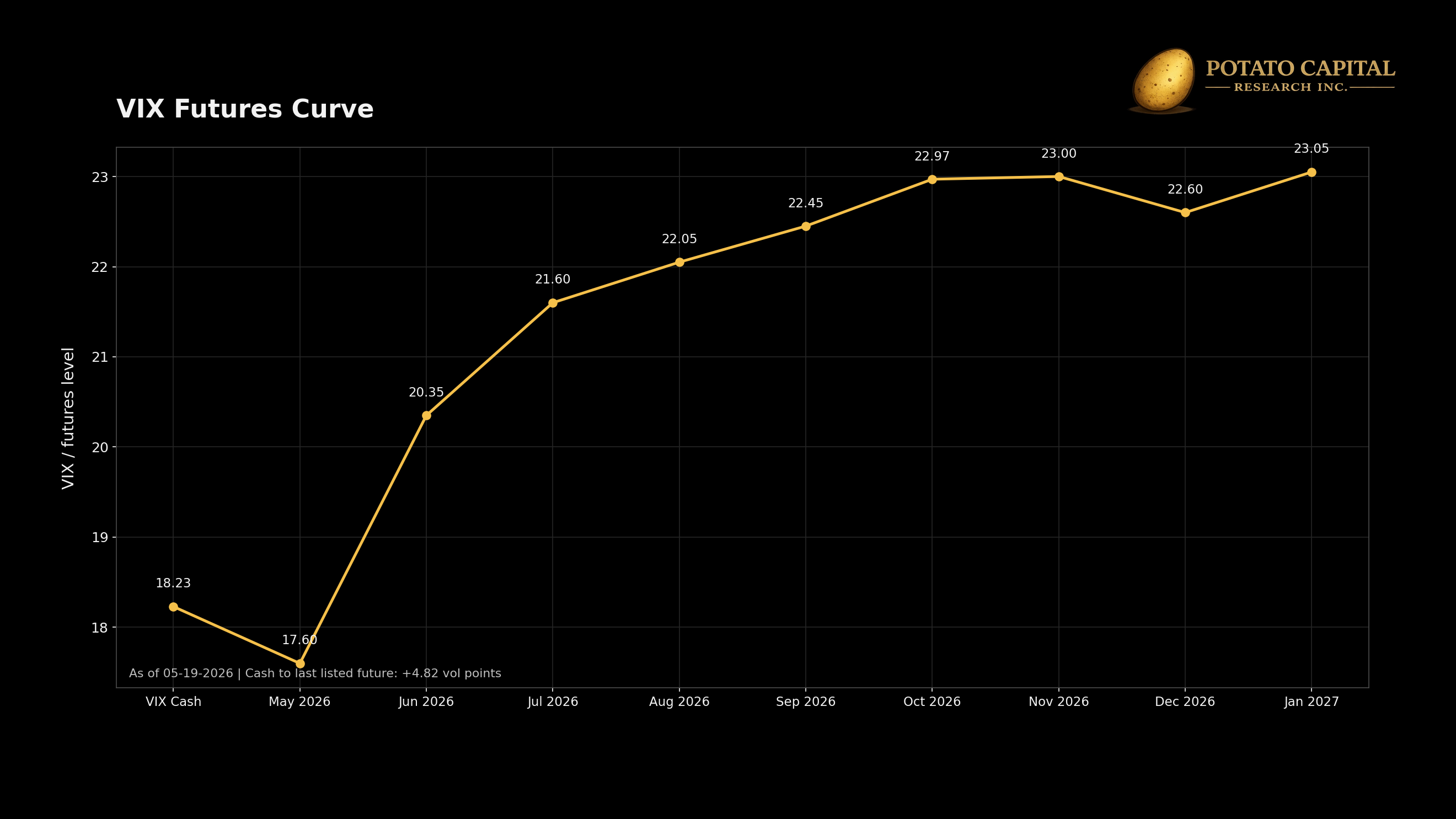
The VIX futures curve also argues against immediate crash pricing. VIX cash was 18.23 on May 19, while June VIX futures traded at 20.35, July at 21.60, and September at 22.45. The curve is upward sloping, which usually points to investors paying for forward volatility risk rather than chasing urgent near-term crash protection. In sharper stress windows, the front end tends to spike and the curve can invert.
Taken together, the options market is pricing three things: a wider distribution for QQQ than SPY, a persistent premium for downside protection, and forward volatility risk without acute front-end panic. That fits the broader setup of the note. The left tail is being priced, but current options data still suggests the market believes the risk is manageable rather than already breaking.
🏛️ Macro Decides which Tail Dominates
Macro conditions can change which tail matters most. Long-duration bonds can protect a portfolio during recessionary disinflation, but they can become a drawdown source when inflation, real rates, or term premium move higher. Commodity producers can look like ordinary cyclicals in a normal slowdown, then become right-tail instruments when supply tightens and spot prices move above the cost curve. The asset label matters less than the shock it is exposed to.
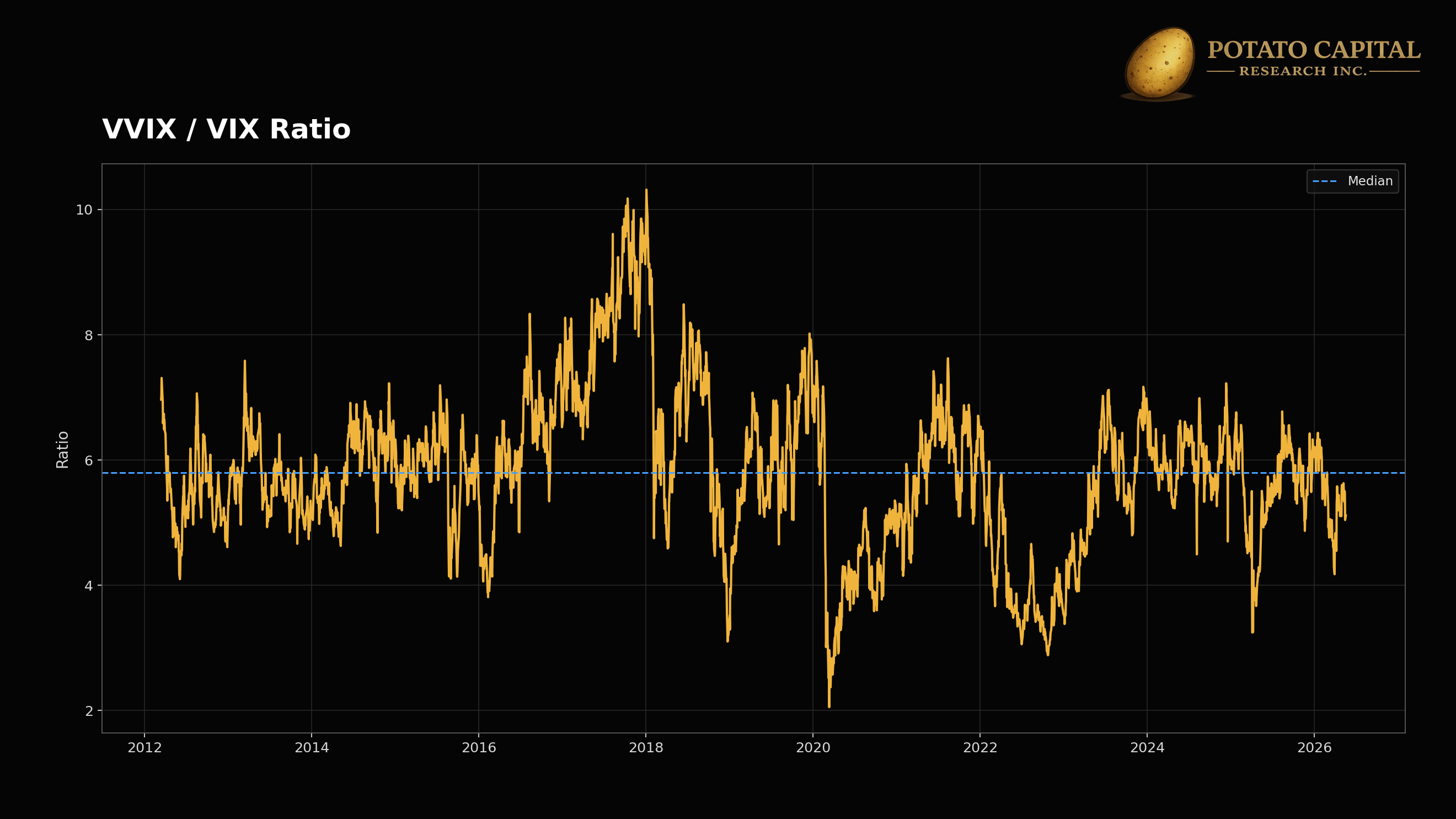
The current dashboard shows priced risk without the pattern of broad systemic stress. VIX was 17.82, VVIX was 91.18, MOVE was 79.87, high-yield option-adjusted spread was 2.8%, and the Chicago Fed National Financial Conditions Index was -0.524 (loose conditions). Credit spreads and funding conditions were still functioning; which matters because a full left-tail credit event usually comes with a wider cluster: higher equity volatility, higher rates volatility, wider credit spreads, tighter financial conditions, and equity drawdowns reinforcing one another.

The current vulnerability is more subtle. Margin debt is elevated, QQQ carries a wider implied distribution than SPY, downside skew remains present, and long-duration assets have already shown they can lose money quickly when rates move against them. A 2.8% high-yield spread does not point to credit panic, but it also leaves less room for complacency if spreads start widening from tight levels while equities are still priced for resilience.
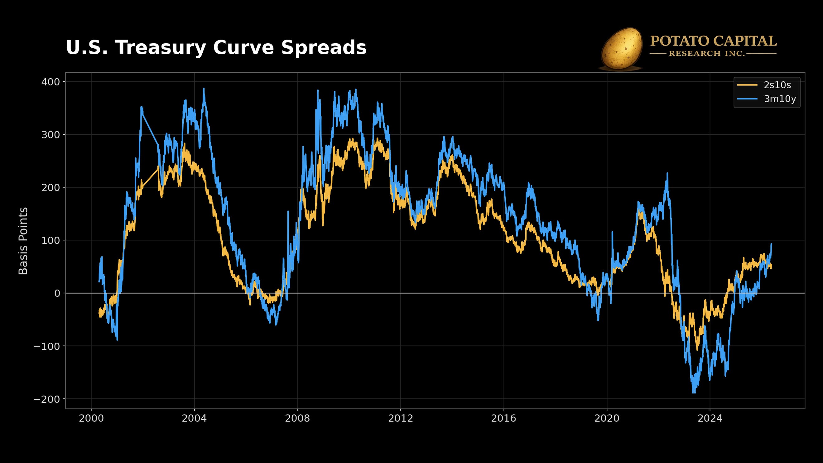
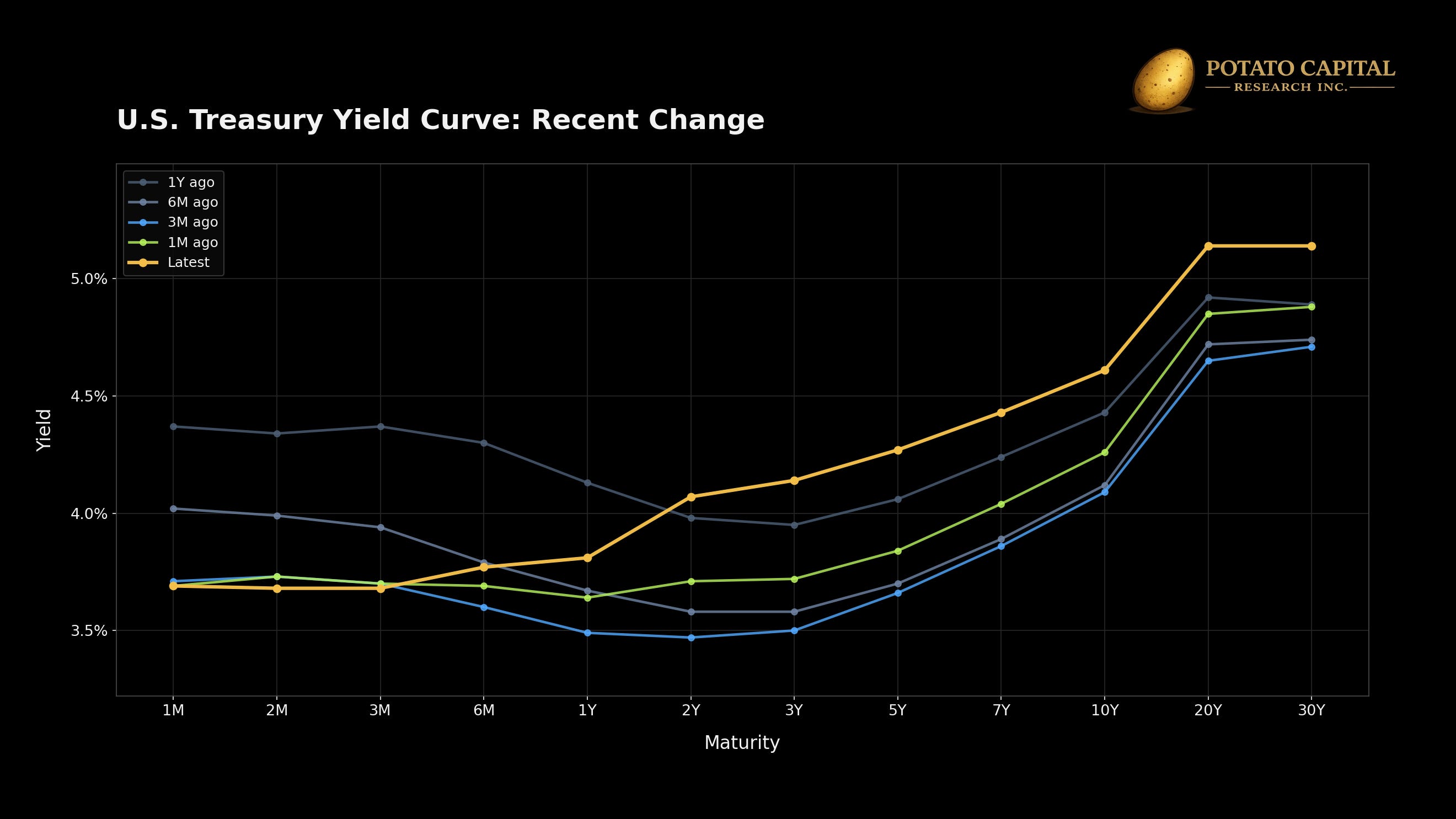
Rates remain the clearest macro pressure point. The 10-year Treasury yield was 4.61%, the 2s10s spread was +54 bps, and the 3m10y spread was +93 bps. A positive curve removes the old inversion signal, but the composition matters. If steepening comes from the long end, higher discount rates can pressure long-duration equity multiples even while credit spreads remain contained.
This is why duration needs regime discipline. In a recessionary disinflation shock, duration can still work as a hedge. In an inflation, real-rate, or term-premium shock, it can become part of the left tail. The 2020 to 2023 bond drawdown already showed that “safe” duration can create portfolio damage without any credit impairment.
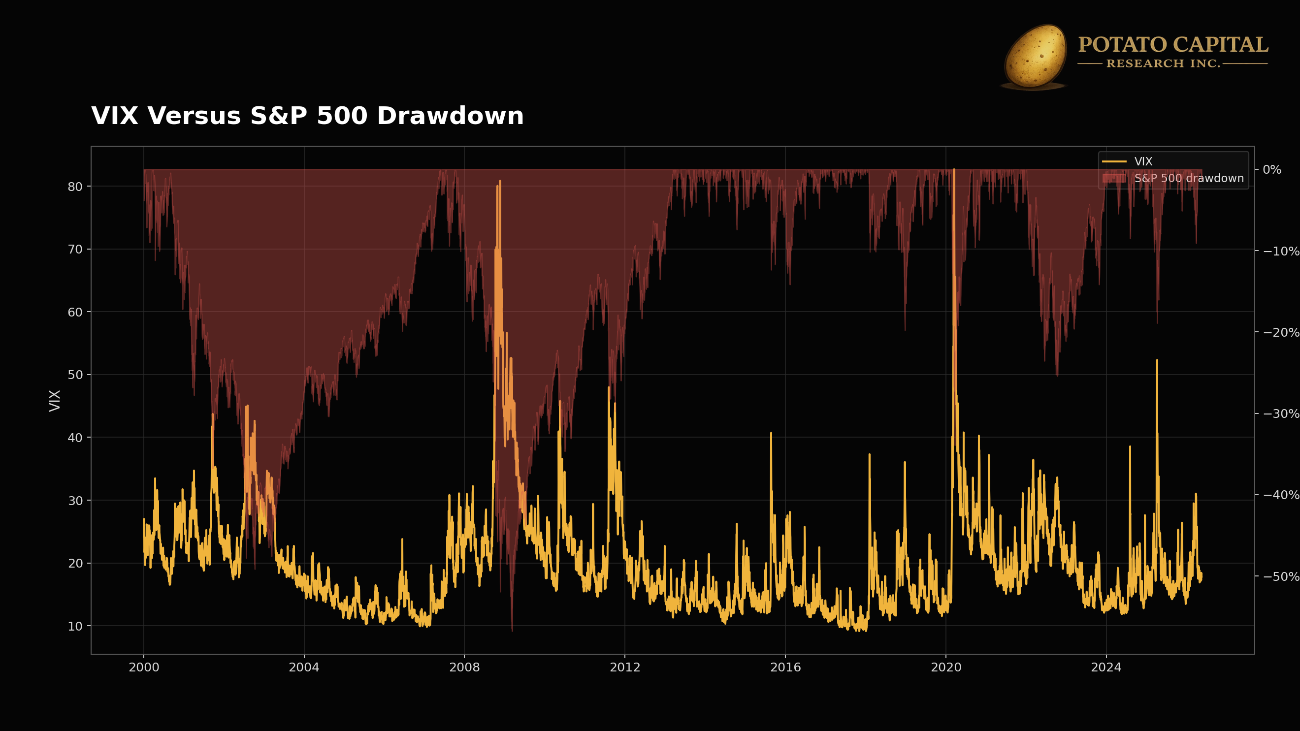
Volatility is the monitoring bridge between macro and portfolio construction. VIX alone is not enough, but a rising VIX alongside rising VVIX, rising MOVE, wider high-yield spreads, tighter financial conditions, and equity weakness would be a much more serious signal. That cluster would suggest the market is moving from priced risk toward forced de-risking.
Disinflation plus easing favors duration and quality growth. Inflation shocks favor real assets and pressure long-duration bonds and high-multiple equities. Credit stress hits cyclicals, small caps, banks, and levered balance sheets. Liquidity booms favor high beta and momentum, while liquidity withdrawal punishes the same exposures. Commodity supply shocks create upside for producers and pressure consumers. Recessions usually hit earnings first, with Treasuries helping only if inflation falls enough to pull rates lower.
The practical takeaway is that macro hedges need to match the shock. Duration hedges recessionary disinflation better than inflation shocks. Commodities hedge supply and currency stress better than demand destruction. Credit spreads can stay calm until refinancing risk suddenly matters. The signal to watch is the combination of higher equity volatility, higher rates volatility, wider spreads, tighter financial conditions, weaker liquidity, and equity drawdowns arriving together.
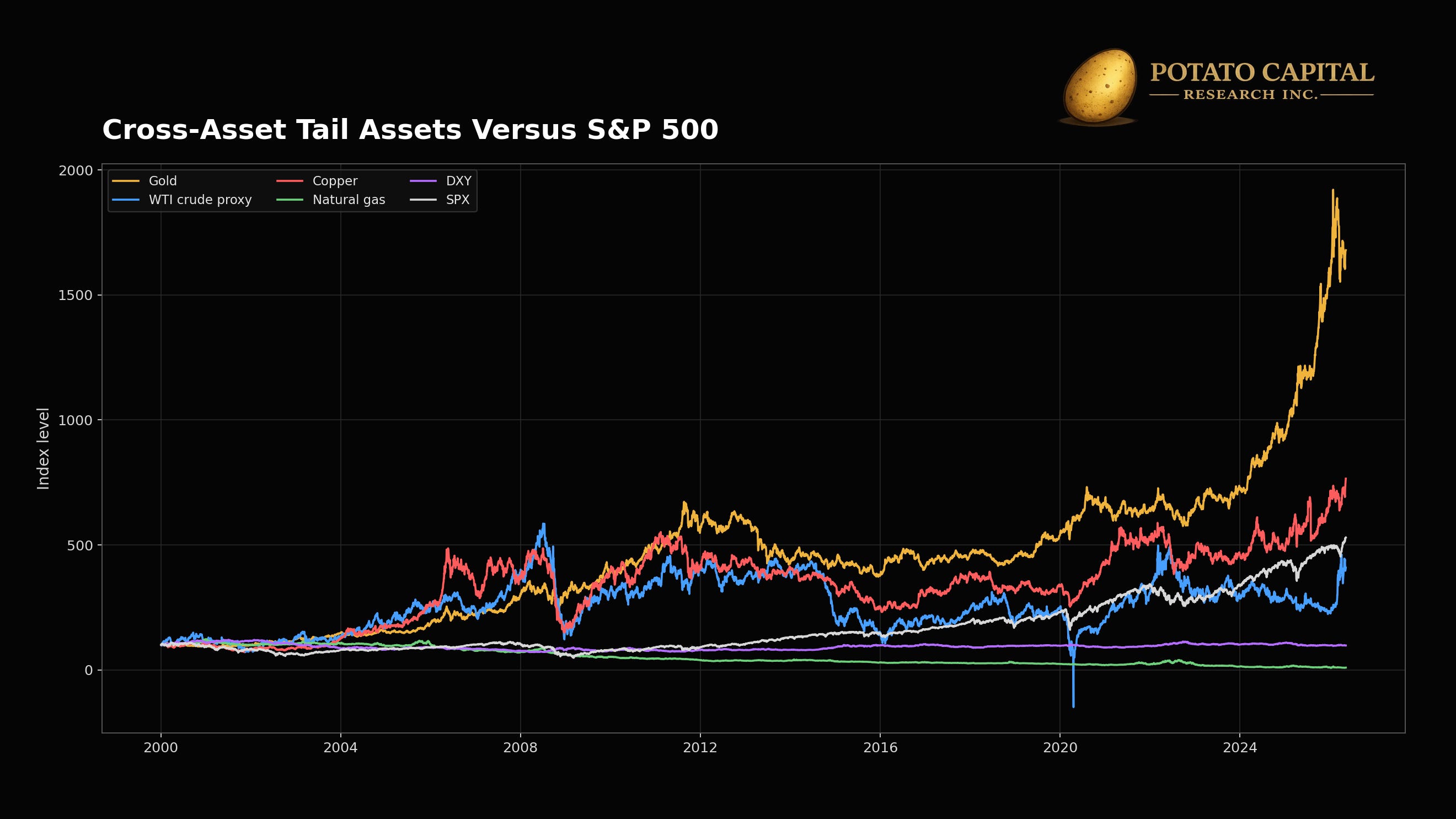
🧮 Cross-Asset Evidence
Cross-asset diversification only works when the return drivers actually differ. The evidence below shows why broad labels like equities, bonds, gold, and factors can hide very different drawdown profiles.
The S&P 500 daily price series since 2000 annualized at 6.4% with 19.3% volatility, but the path included a -56.8% maximum drawdown. IWM had a worse profile: 23.9% annualized volatility and a -59.9% maximum drawdown. Small caps carry more than equity beta. They are more exposed to financing conditions, domestic cyclicality, and liquidity withdrawal, which makes the left tail deeper when credit and liquidity conditions deteriorate together.
TLT’s daily history since July 2002 shows a -48.4% maximum drawdown from August 2020 to October 2023, with no full recovery yet. IEF drew down -27.7% over the same peak-to-trough window. The mechanism was rate sensitivity. Long-duration Treasuries can still work in recessionary disinflation, but inflation and rate repricing turned them into a source of portfolio drawdown.
Gold’s daily series showed a 10.7% annualized price return since 2000 with 17.1% annualized volatility and a -44.6% maximum drawdown from September 2011 to December 2015. That is the cost of owning a regime-sensitive hedge. Gold can help when the shock is currency, inflation, or confidence-related. It can also drag for years when real rates, dollar strength, and risk appetite move against it.
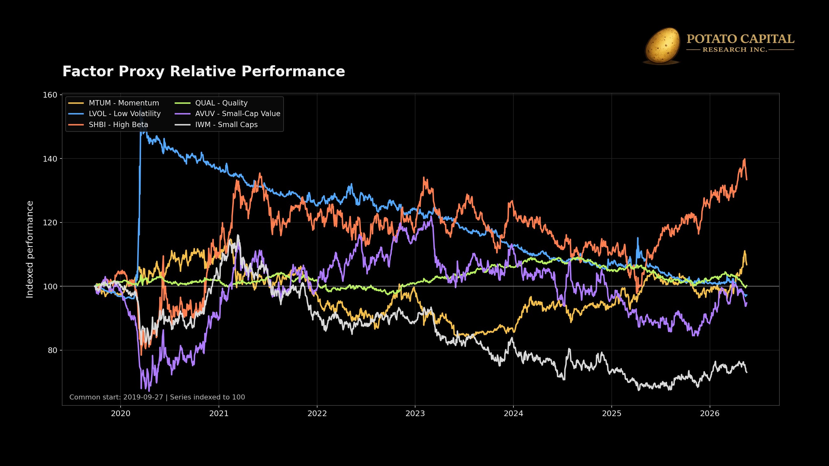
The factor data shows the same tradeoff inside equities. From September 27, 2019 to May 18, 2026, high beta outperformed the S&P 500 by 33.4% on a relative basis, but it also had a -47.2% maximum drawdown. Low volatility lagged the S&P 500 by 2.8%, but its maximum drawdown was much smaller at -24.8%. Quality roughly matched the S&P 500 over the period with a -34.1% maximum drawdown.
Small caps, high beta, and long-duration growth can look diversified by ticker while sharing sensitivity to liquidity and rates. Duration can hedge one macro regime and hurt in another. Gold can diversify one shock and drag through another. Portfolio construction has to start with the tail being hedged, not the asset label.
🔁 Portfolio Construction: Owning the Tails Deliberately
A tail-aware portfolio starts with the failure path: what has to be sold, refinanced, hedged, or resized if the bad state arrives first? The key questions are where the book can suffer forced losses, where it owns genuine upside convexity, where it is implicitly short volatility, and where liquidity could disappear when markets stop trading cleanly?
The evidence points to a few rules. The S&P 500’s drawdown history shows that path matters. TLT and IEF show that duration can become a drawdown source when the shock is inflation and rate repricing. FINRA margin debt shows why leverage can make a correction more fragile. The factor data shows that high beta can deliver stronger upside with a much deeper drawdown profile. Company data shows that right-tail upside is higher quality when it comes with free cash flow conversion and limited dilution.
The core of the portfolio should be built around assets that can survive the left tail without forced dilution, refinancing pressure, or thesis breakage. In equities, that usually means durable cash flow, manageable leverage, high returns on capital (ROIC, ROCE), and reinvestment that does not depend on permanently loose funding conditions. The core does not need to lead every rally. Its job is to keep compounding when volatility rises and capital becomes more selective.
Right tail exposure should be explicit and sized around the path, not the payoff headline. Long-dated options, distressed recoveries, commodity torque, product inflections, and high-beta exposures can all have a role, but the evidence has to justify the risk budget. It would be imprudent to put a whole portfolio in options. CVNA shows how large the payoff can be when equity survives, while the -99% drawdown shows why that type of exposure cannot be treated like a normal core holding. FCX shows that commodity torque can pay, but the drawdown profile belongs in a cyclical sleeve. PLUG and BYND show why revenue growth without cash conversion or dilution control deserves a much higher burden of proof.
The hedge sleeve should match the actual risk in the portfolio: index puts or collars can help when the portfolio is exposed to broad equity beta; cash and bills protect flexibility; duration can hedge recessionary disinflation; gold and commodities can help against inflation, supply, and currency shocks (but they can also carry long holding-period drawdowns). The hedge has to match the regime and the vulnerability.
Liquidity deserves its own budget. Cash and short-term bills are not idle if they prevent forced selling, allow rebalancing into liquidation pressure, and keep right-tail positions alive when markets reprice risk. That matters more when margin debt is elevated and options markets are still charging a premium for downside protection.
Position sizing should follow the job of the position. Durable cash-flow compounders can carry larger weights if valuation still leaves enough forward return. Commodity torque belongs in a cyclical sleeve. Distressed equity and long-dated options should be small enough to fail without damaging the portfolio. Hedges should be judged against the tail they are meant to cover, not against equity returns in every month.
What happens if the bad state arrives before the good state? If the answer is forced selling, dilution, refinancing stress, or a position size that cannot be held through the drawdown, the exposure is too large for the role it plays in the portfolio.
🥔 Final Take
The market’s long-run return is real, but it is only available to capital that can survive the full cycle path. Since 2000, the S&P 500 annualized positively while carrying fat-tailed daily losses, a -56.8% maximum drawdown, and several regimes where the source of risk changed completely. A portfolio that cannot absorb those transitions does not get to enjoy the average.
The upside tail needs the same discipline. NVDA and META show what higher-quality right-tail exposure looks like: growth that translated into cash conversion, margin expansion, and shareholder returns. CVNA and FCX show more volatile versions, where the payoff was real but the drawdown profile required tighter sizing. PLUG and BYND show the failure case: revenue narrative without durable cash economics or dilution control.
The current market is showing vulnerability rather than full-system stress. Credit spreads remain contained, financial conditions are still loose, VIX futures are upward sloping, and implied volatility is below crisis levels. The weaker points are more specific: margin debt is elevated, downside skew remains present, QQQ carries wider implied path risk than SPY, and long-duration assets have already shown how quickly “safe” exposures can become drawdown sources when inflation and rates move against them.
Portfolio construction should follow that evidence. Durable cash-flow assets can sit in the core if valuation still leaves enough forward return. Right tail exposures belong in sleeves sized around their drawdown path, not the size of the upside story. Hedges need to match the shock being hedged: duration for recessionary disinflation, real assets for inflation and supply stress, index protection for broad beta, and cash for liquidity when forced sellers appear.
The goal is to know which tail the portfolio is being paid to hold, whether the price is reasonable, and whether the position size can survive the path required for the thesis to work.
Sources: Barchart, S&P Dow Jones Indices, Cboe Global Markets, Nasdaq, FINRA, Federal Reserve Bank of St. Louis, Federal Reserve Bank of Chicago, ICE BofA Indices, U.S. Treasury, CME Group, and ETF issuer price histories.